The state‐space representation is a useful tool for analysing many dynamic models. When this representation exists, the Kalman filter can be applied to estimate the model parameters, to compute predictions or to smooth the series. This technique was introduced by Kalman (1960) in the field of engineering but has been used in various domains, in particular in economics.

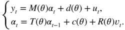
We first introduce state‐space representations and useful notations. Let (y _t ) denote a ℝ ^N ‐valued observable process, and let (α _t ) a ℝ ^m ‐valued latent (in general non‐observable, or only partially observable) process. A state‐space model is defined by

D.1

where M _t , d _t , T _t , c _t and R _t are deterministic matrices of appropriate dimensions, (u _t ) and ( ) are white noises, respectively, valued in ℝ ^N and ℝ ^m . The vector α _t is called space vector. The first equation is called measurement equation, and the second equation transition equation.

The Kalman filter is an algorithm for

1. (i) predicting the period‐ t space vector from observations of y up to time t − 1;
2. (ii) filtering, that is predicting the period‐ t space vector from observations of y up to time t ;
3. (iii) smoothing, that is estimating the value of α _t from observations of y up to time T , with T > t .

In this appendix, we present basic properties of the Kalman filter. The reader is referred to Harvey (1989) for a comprehensive presentation of structural time series models and the Kalman filter.

In order to implement the algorithm, we make the following assumptions.

• The process (u _t , ) is an iid Gaussian white noise such that
  D.2
• The initial state vector is Gaussian and is independent from the noises (u _t ) and ( ):
  
• For all t , the matrix H _t is positive‐definite.

  These assumptions imply, in particular, that the variables u _t and are independent from (y ₁, y ₂, …, y _t − 1). Assuming non‐correlation of u _t and is not essential, as we will see, but allows us to simplify presentation. The assumption that H _t is positive‐definite can be very restrictive (in particular when the noise of the measurement equation is degenerate), but it is not necessary. It is introduced to ensure the positive‐definiteness of the conditional variance of y _t given y ₁, …, y _{t − 1 .}

  The algorithm allows to recursively compute the conditional distribution of α _t given y ₁, …, y _t . This distribution is Gaussian and its mean provides “estimator” of de α _t which is optimal (in the L ² sense). When the Gaussian assumption is in failure, the Kalman filter no longer provides the conditional expectation of α _t . The resulting estimator is no longer optimal, but only optimal among the linear estimators.

D.1. General Form of the Kalman Filter

The derivation of the algorithm requires the following notations:

The first two equalities hold t ≥ 1, the other two ones for t > 1. Let α _1 ∣ 0 = E(α ₁) and P _1 ∣ 0 = Var(α ₁).

First Step

By taking the conditional expectation with respect to y ₁, …, y _t − 1 in the transition equation, we get

D.3

and then, by taking the conditional variance,

D.4

Such equations are called prediction equations.

The conditional moments of y _t follow:

D.5

and

D.6

We will also use

D.7

Second Step

Once the observation y _t becomes available, the preceding quantities are updated:

D.8

and

D.9

Such equations are called updating equations.

The normality assumption is only involved in the second step. Indeed, we use the fact that the distribution of (y _t , α _t ) is Gaussian conditional on y ₁, …, y _t − 1 ¹

which allows to derive the law of α _t conditional on y ₁, …, y _t − 1, y _t . ²

Initial Values of the First Step

The starting values for the Kalman filter can be specified by noting that the conditional and unconditional moments coincide:

D.10

The quantities α _{t ∣ t − 1} , P _{t ∣ t − 1 ,} and α _t ∣ t , P _t ∣ t can thus be recursively computed for t = 1, …, n .

To summarise, the Kalman filter is an algorithm for computing the sequences and , where α _{t ∣ t − 1} denotes the optimal prediction of the state vector α _t given the observations y ₁, …, y _t − 1 . The mean squared error for this prediction is . These sequences can be directly obtained from the following formulas, which follow from substituting formulas (D.8) and (D.9), taken at t − 1, in (D.3) and (D.4):

D.11

and

D.12

where

D.13

It can be noted that the sequence does not depend on the observable variables, and can be computed independently from the sequence . Matrix K _t is called the gain matrix.

D.2. Prediction and Smoothing with the Kalman Filter

Prediction

The Kalman filter can be used for prediction at horizon larger than 1. To simplify presentation, let us assume that c _t  = d _t  = 0, T _t  = T and M _t  = M for all t . We thus have, for any integer h ,

and, consequently,

The variance of the prediction error at horizon h + 1 is given by

From these equations, we deduce the predictions of the observed process. We have y _t + h  = Mα _t + h  + u _t + h and thus

The prediction error is y _t + h  − y _{t + h ∣ t − 1} = M(α _t + h  − α _{t + h ∣ t − 1}) + u _t + h and the corresponding mean‐square error is

Smoothing

Formula (D.8) gives the smoothed value α _t ∣ t of α _t , that is, its prediction given the observations up to period t . In some applications, the value of the state vector is of prime interest, and one may want to predict its values a posteriori. Smoothing techniques use observations posterior to period t to predict α _t . Let

where n is the sample size.

The smoothed values can be computed as follows. First, apply the Kalman filter to the data, and compute the sequences (α _t ∣ t ) and (P _t ∣ t ) from (D.8) and (D.9), as well as the sequences (α _{t ∣ t − 1}) and (P _{t ∣ t − 1}), obtained from (D.3) and (D.4). Then, the following algorithm – initialised at α _n ∣ n – is used to compute in a descending recursion the α _t ∣ n 's. The equations are

D.15

and

D.16

where

Note that the variance‐covariance matrices P _t ∣ n can be computed independently from the data, and that the smoothed vectors α _t ∣ n are linear combinations of the observations (with coefficients depending on t ).

To establish such formulas, we use the fact that the law of (y _t , α _t , α _t + 1) conditional on y ₁, …, y _t − 1 is Gaussian. It follows that, using again the property of multivariate normal vectors, the conditional law of α _t given α _t + 1, y ₁, …, y _t is Gaussian with mean

because

Next, we note that, for predicting α _t , the knowledge of y _t + 1, …, y _n does not convey additional information with respect to α _t + 1, y ₁, …, y _t . Indeed, the variables y _t + j , j > 0 can be written as linear combinations of α _t + 1, u _t + j , _t + 2, …,  _t + j . The prediction error α _t  − E(α _t  ∣ α _t + 1, y ₁, …, y _t ) is – by definition – orthogonal to α _t + 1 , and also to the future noise values. We thus have,

D.17

By the iterated projection formula, it now suffices to take the expectation of both sides of this equality conditional on y ₁, …, y _n to get (D.15) (noting that the variables α _t ∣ t and α _{t + 1 ∣ t} are functions of the observables).

In order to compute the mean squared error, we note that the smoothing error is

Therefore,

and hence,

D.18

In this expression, the autocovariances are equal to zero because α _{t + 1 ∣ n} (resp. α _{t + 1 ∣ t} ) is a linear combination of the observations, and thus is orthogonal to the error α _t  − α _t ∣ n (resp. α _t  − α _t ∣ t ). Moreover, the smoothing error α _t + 1 − α _{t + 1 ∣ n} being orthogonal to α _{t + 1 ∣ n} , we have Cov(α _t + 1, α _{t + 1 ∣ n} ) = Var(α _{t + 1 ∣ n} ) thus

Similarly, Var(α _{t + 1 ∣ t}  − α _t + 1) = Var(α _t + 1) − Var(α _{t + 1 ∣ t} ), therefore,

Combining the equation with (D.18) we get (D.16).

Note that, as for the Kalman filter formulas, the smoothing formulas remain valid without normality of the errors but only provide, in this case, linear expectations of the state vector.

D.3. Kalman Filter in the Stationary Case

It is worth considering the asymptotic behaviour, when t goes to infinity, of the Kalman filter formulas. Let us focus on the model with constant coefficients and constant variance‐covariance matrices

D.19

The state vector α _t is thus the solution of a first‐order Vectoriel Autogregressive (VAR(1)) model. This model admits a second‐order stationary solution if the spectral radius ρ(T) of matrix T is strictly less than 1. Under this assumption, the first two moments of the stationary solution satisfy

D.20

where

If the initial distribution of the state vector, , is such that a ₀ = (I − T)⁻¹ c and vec(P ₀) = (I − T ⊗ T)⁻¹vec(RQR ^′), then (D.20) holds for any t ≥ 0 _.

Interestingly, under the stationarity assumption, the sequence (P _{t ∣ t − 1}) defined by (D.12) converges. Indeed, let us first note that this formula reduces to

D.21

where

If the latter sequence converges, the limit P ^* = lim P _{t ∣ t − 1} necessarily satisfies

D.22

See for instance dans Hamilton (1994, Section 13.5) for a proof. Note that (D.22) is called algebraic Ricatti equation. An explicit solution for this equation is seldom available and, moreover, the solution may not be unique. It can be shown that when P ^* is the unique solution, the sequence (P _{t ∣ t − 1}) converges at exponential rate (see Harvey 1989 and references, Section 3.3.3).

From a numerical point of view, the convergence of the sequence (P _{t ∣ t − 1}) _t ≥ 1 may be worthwhile. Notice that the sequence (F _{t ∣ t − 1}) and (K _t ) defined in (D.13) also converge in this case, with respective limits

D.23

When P _{t ∣ t − 1} is sufficiently close to the limit P ^* , formula (D.11) updating the predictions of α _t can be approximated by

D.24

The saving in the computation time may be very large when this approximation is used, because it allows to avoid the inversion of the – possibly high‐dimensional – matrix F _{t ∣ t − 1} , at every step of the algorithm. Once the limit is close to be reached, the inverse of the matrix F ^* can be used instead of . Equation (D.21) thus become useless. A criterion for stoping the computations of P _{t ∣ t − 1} can be based on the determinant of this matrix: for instance, the approximation can be used if ∣ det P _{t + 1 ∣ t}  − det P _{t ∣ t − 1} ∣  < τ where τ is a very small positive number.

D.4. Statistical Inference with the Kalman Filter

In this section, we assume that the matrices M _t , d _t , T _t , c _t , and R _t of the state space model are constant and are parameterised by a vector θ belonging to a parameter set Θ ∈ ℝ ^d . The state‐space representation thus has the form

D.25

We also assume that the joint Gaussian distribution of the noise is time‐independent, but may depend on θ :

D.26

From observations y ₁, …, y _n , and for given functions M, d, T, c, H and Q , the problem is to estimate θ . Conditional on initial values ε ₁(θ) and F ₁(θ), the Gaussian likelihood L _n (θ) writes

where, for t > 1, ε _t (θ) = y _t  − E _θ (y _t  ∣ y ₁, …, y _t − 1), F _t (θ) = Var _θ (y _t  ∣ y ₁, …, y _t − 1) and ∣A∣ denotes the determinant of a square matrix A . Expectations and variances indexed by θ mean that they are computed as if θ was the true parameter value.

A maximum likelihood estimator (MLE) of θ is defined as any measurable solution of

By taking the logarithm, maximising the likelihood with respect to θ amounts to minimising

D.27

The Kalman filter allows us to compute ε _t (θ) and F _t (θ), for any value of θ , when such quantities cannot be easily obtained. Numerical optimisation procedures can be used to obtain the optimum parameter value. The theoretical properties of the MLE (consistency, asymptotic normality) require additional assumptions on the observed process and the parameter space, which will not be detailed here.