
Chapter 8. Black Hole Simulations with CUDA
Frank Herrmann, John Silberholz and Manuel Tiglio
In 1915 Albert Einstein derived the fundamental laws of general relativity that predict the existence of gravitational radiation. While indirect evidence is by now well established and led in 1993 to the Nobel Prize in Physics being awarded to Russel A. Hulse and Joseph H. Taylor, no direct detection has occurred to date. This is because gravitational waves reaching Earth are extremely weak. Recently, researchers have built gravitational wave detectors achieving the required sensitivities to make direct detection possible. A number of laser interferometer experiments are devoted to this task. The currently most sensitive one (LIGO
[1]
) consists of two crossed laser beams, each of which is 4km long. Over this distance a typical gravitational wave would change each arm's length by
 m — a fraction of the size of an atom. Because the signal to be extracted is very small compared with the background noise, an accurate a priori knowledge of inspiral signals that can be searched for in the data is required.
In this chapter we discuss our CUDA and GPU implementation and results from an approximation to Einstein's equations, the
post-Newtonian
one, which allows us to thoroughly study the inspiral phase-space dynamics of the seven-dimensional parameter space of binary black holes in initial quasi-circular orbit.
8.1. Introduction
With a number of gravitational wave detectors such as LIGO
[1]
, Virgo
[2]
and GEO600
[15]
now measuring at design sensitivity, the prospect of direct detection of gravitational radiation is becoming increasingly real. Because of the low signal-to-noise ratio encountered at these detectors, researchers need to post-process the data, ideally searching for known signals that would indicate a source of gravitational radiation. One of the most likely sources of detection are stellar-mass binary black hole (BBH) systems. There is a definite need to understand as much as possible about these configurations.
Over recent years numerical solutions of general relativity (GR) have reached the point where accurate and reliable calculations of the interactions of two black holes (BHs) over many orbits can be produced by a number of different groups
[3]
[4]
and
[12]
. These calculations require enormous computational effort, though, and the generation of a large-scale bank of numerical templates that could be used by gravitational wave detectors is currently intractable. Numerical solutions to Einstein's equations require solving a coupled set of nonlinear elliptic-hyperbolic partial differential equations in three spatial dimensions. A single right-hand-side call to advance in time just one point on the three-dimensional
spatial grid requires around 13,000 multiplications, 5400 additions, 3400 subtractions, and 69 divisions, excluding derviative calculations. A single simulation can easily take more than 100,000 CPU hours. These simulations are typically running on more than 1024 cores simultaneously so that they can complete in a reasonable amount of time. Here, we report on an approximation to GR, the so-called post-Newtonian expansion (PN), which — as explained in the next section — dramatically reduces the number of computational operations required. Furthermore, recent comparisons between gravitational waveforms obtained from full numerical relativity (that is, numerical solutions of the full Einstein equations) and PN approximations show good agreement until just a few orbits before the two black holes merge
[5]
[8]
and
[13]
.
Because of these reasons, performing a large number of PN simulations of BBH systems with different initial configurations is of considerable interest, and it is the focus of our work described in this chapter.
8.2. The Post-Newtonian Approximation
The PN approximation leads to a system of coupled ordinary differential equations (ODEs) in time for the orbital frequency
 , the unit orbital angular momentum vector
 and the individual spin vectors
 for the two BHs. This expansion is valid as long as the two black holes are far separated and slowly moving along a quasi-circular inspiral trajectory. In total this is a seven-dimensional problem as there are three degrees of freedom in each of the spin vectors and one degree of freedom in the mass ratio.
The specific PN expansion and equations that we use are those of Ref.
[6]
(with Erratum
[7]
); namely,
(8.1)
(8.2)
(8.3)
The evolution of the individual spin vectors
 for the two BHs is described by a precession around
 ,
Eq. 8.2
, with
,
Eq. 8.2
, with
 and
and
 obtained by the exchange
 . The spin vectors
 are related to the unit ones
 via
via
 , with
 the dimensionless spin parameter of each black hole.
(8.4)
8.3. Numerical Algorithm
The ODEs are integrated in time using Dormand-Prince's method
[10]
. This ODE integrator uses an adaptive time step
 to keep the solution error below a given threshold. Starting from time
 , the time integrator updates the state to
 . It computes an approximation to the solution at six intermediate times between
 and
and
 (referred to as
k1
to
k6
later in this chapter) and then computes fourth-order and fifth-order accurate solutions at
(referred to as
k1
to
k6
later in this chapter) and then computes fourth-order and fifth-order accurate solutions at
 (here denoted
y4
and
y5
). This requires six right-hand-side calls, that is, six evaluations of the right-hand-sides of
Eqs. 8.1
–
8.3
. The difference between these solutions is used to estimate the error of
y4
and adapt
(here denoted
y4
and
y5
). This requires six right-hand-side calls, that is, six evaluations of the right-hand-sides of
Eqs. 8.1
–
8.3
. The difference between these solutions is used to estimate the error of
y4
and adapt
 if the error is below some specified tolerance. In our simulations we typically set the tolerance to be
 (i.e., roughly at the level of single-precision accuracy) and start with an adaptive time step of size
 . The time step does not change during most of the inspiral. This is crucial for our GPU implementation because — as discussed later in the chapter — it minimizes thread divergences when multiple inspirals are performed in parallel.
Each ODE integration described earlier in this chapter cannot be easily parallelized because the solution at each time step (even for the intermediate
k1
to
k6
values) depends on the previous one. However, if one wants to study an ensemble of BBH inspiral dynamics (for example, in a phase-space study), then a trivial parallelization is available by just performing many inspirals simultaneously.
Figure 8.1
shows a CUDA pseudo-code description of our implementation. The right-hand-side (RHS) expressions of
Eqs. 8.1
,
8.2
and
8.3
are implemented in the
ode_rhs
function on the GPU. The ODE integration is performed on the CPU. First, GPU storage is allocated in
allocate_gpu_storage
. Then, the initial state data (i.e.,
 ,
,
 for the two BHs, and the unit orbital angular momentum vector
 ) is set. In the evolution loop the RHS is called, and the different intermediate values
k1
to
k6
are computed in
interm_1
, etc. Next, for each inspiral the time step
) is set. In the evolution loop the RHS is called, and the different intermediate values
k1
to
k6
are computed in
interm_1
, etc. Next, for each inspiral the time step
 is adjusted separately; that is,
 is a vector with entries for each parallel inspiral. Finally, the loop is terminated once all the physical configurations have reached a final frequency
 to a given precision. At the end the data is copied back from the GPU to the CPU. During each time step a memory copy from the GPU to the CPU is needed to check if all simulations are done. In the profiling
Section 8.5
we will see that no significant amount of time is spent in this copying.
to a given precision. At the end the data is copied back from the GPU to the CPU. During each time step a memory copy from the GPU to the CPU is needed to check if all simulations are done. In the profiling
Section 8.5
we will see that no significant amount of time is spent in this copying.
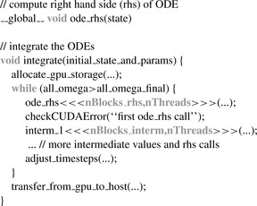 |
| Figure 8.1
Pseudo-code describing the parallel ODE integration. The time integration is performed on the CPU with kernels performing the inspirals called on the GPU as described in the text.
|
Unfortunately, BBH systems interact differently based on their initial state, which describes their relative masses and the orientations of their spins. In particular, this will lead to thread divergence of the different inspirals. This could potentially be a very serious problem as time steps are adjusted in different manners and the load/store patterns of the different threads running in parallel changes. In our simulations we have found, however, that the divergence in the threads appears only toward the very end of the inspirals as only then are the time steps adjusted in a dynamic manner, typically resulting in a runtime difference of at most 10% from just running many copies of the same inspiral. This simplifies the problem significantly, as we do not have to handle thread divergence.
GPUs today provide the most impressive speedups over CPUs for single-precision computations. By comparing single-precision and double-precision CPU results on a number of inspiral configurations,
we have verified that single-precision processing is sufficient for our problem, yielding a maximum error of just over
 for any final parameter after the simulation, sufficient for our studies.
8.5. Performance Results
We now evaluate the performance advantages GPUs deliver in our application. We executed our code on a single core of a quad-core Intel Xeon E5410 CPU running at 2.33GHz, which is rated at around 5GFlops in double-precision. Note that the problem is embarrassingly parallel, and therefore, the CPU would be able to provide excellent scaling over its four cores. We integrated one of our test inspirals 100 times serially and found that we could achieve around 0.057 inspirals per millisecond (ms) on a single core — which we will use for our performance comparison.
For comparison, each of the four GPUs on a high-end unit (the NVIDIA Tesla S1070) is currently rated at 1035GFlops in single-precision, delivering a theoretical performance advantage of about a
factor 200
over the single-core CPU. We ran our test setup on a single GPU, spawning a large number
 of simultaneous inspirals in parallel.
Figure 8.2a
shows results for the performance of the GPU card. As we increase the number of simultaneously scheduled inspirals
of simultaneous inspirals in parallel.
Figure 8.2a
shows results for the performance of the GPU card. As we increase the number of simultaneously scheduled inspirals
 the speed levels off at about 2.7inspirals/ms. The GPU has 240 processors that work in parallel, but the runtime CUDA scheduler has to be able to keep these 240 processors working simultaneously by switching out threads that would pause while waiting for a memory access to complete. This is the reason why the performance still rises even after
 , as the runtime has a better chance of squeezing the optimal performance out of the card by interleaving different inspirals without having to wait for costly memory transfers.
Figure 8.2b
shows more detailed profiling information. Listed is the time spent on different routines for one of our simulations run with
, as the runtime has a better chance of squeezing the optimal performance out of the card by interleaving different inspirals without having to wait for costly memory transfers.
Figure 8.2b
shows more detailed profiling information. Listed is the time spent on different routines for one of our simulations run with
 ; note the log-scale. The RHS computations dominate, as expected from the arithmetic intensity of
Eqs. 8.1
,
8.2
and
8.3
. The next most expensive routines relate to the time update step. The
y4
and
y5
are the routines performing the estimation updates from the ODE integrator mentioned in
Section 8.3
, the
k1
to
k6
are the routines for the intermediate computations, while
D.to.H
and
H.to.D
refer to device-to-host and host-to-device
memcopy
operations. Finally,
pois.float
,
pois.int
, and
init
are all initialization steps, which are only run once.
; note the log-scale. The RHS computations dominate, as expected from the arithmetic intensity of
Eqs. 8.1
,
8.2
and
8.3
. The next most expensive routines relate to the time update step. The
y4
and
y5
are the routines performing the estimation updates from the ODE integrator mentioned in
Section 8.3
, the
k1
to
k6
are the routines for the intermediate computations, while
D.to.H
and
H.to.D
refer to device-to-host and host-to-device
memcopy
operations. Finally,
pois.float
,
pois.int
, and
init
are all initialization steps, which are only run once.
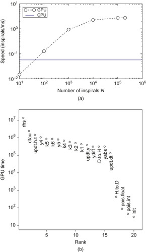 |
| Figure 8.2
Performance of the GPU. Figure a shows scaling as we increase the number of inspirals
N
simultaneously scheduled on the GPU. Figure b shows profiling results — right-hand-side (RHS) computations dominate, as expected.
|
We performed this study using block sizes of 256 threads. We found similar behavior with 128-thread blocks. Based on this data, we achieve a
speedup of about a factor 50
. While this comparison is slightly unfair to the CPU because we only use a single core and double-precision mode on the CPU, there is no doubt that the performance gains are very significant. Note also that for this test problem we integrated the exact same problem in all cases. This means that the individual threads run in perfect lock-step, the best possible case for the GPU. As mentioned earlier in this chapter, we typically see differences of about 10% in the runtime of different inspirals, and this would result in a slight inefficiency on the GPU as some of the threads in a block may finish before others.
8.6. GPU Supercomputing Clusters
To further speed our computations, we used the NCSA Lincoln cluster, which is a cluster of 96 NVIDIA Tesla S1070 units connected to 192 eight-core Dell PowerEdge 1950 servers (each scalar unit allows access to two GPUs). To perform these computations, we used a Message Passing Interface (MPI),
designating one node as a lead node that delegates tasks to others and keeps track of the progress of the overall job. We subdivided each large computation into a set of smaller jobs, which were completed by individual GPUs. To limit network communication overhead, we sent only basic information about the jobs to the nodes performing the computation, and they calculated the parameters for each of the runs
and then performed the computations. On completion of a job, the resulting data file (stored in a binary format to conserve space) was stored on tape storage provided by the cluster. Throughout the course of the run, we would copy files from that storage to a local hard drive so that we had all the files stored locally by the end of the computation.
Several robustness measures were necessary to successfully complete the computation and transfer of the resulting data. Occasionally, a node would never complete a job, blocking completion of the overall computation. To prevent this, we had the lead node reassign abnormally long-running jobs. Further, in our real-time data transfer system, it was sometimes difficult to determine if a file on the tape storage represented a partially or fully transferred data file. To ensure we only copied complete data files to our local hard drive, we added an indicator file to the tape storage to mark that a file had been fully transferred. Last, sometimes our transfers from the tape storage to our local hard drive — using high-performance enabled secure copy (HPN SCP) — only partially completed. We validated the copies by comparing the hash values of the data files on the tape storage to those on the local hard drive.
By using a GPU supercomputing cluster, we were able to significantly speed our investigation on the phase space of a binary black hole system.
8.7. Statistical Results for Black Hole Inspirals
As described in
[14]
, we can gain significant insight into the interactions of BBH systems through a systematic sampling and evolution of the parameter space of initial configurations. In particular, in a recent statistical study
[11]
, through a principal component analysis of our simulation results, we found quantities that are nearly conserved, both in a statistical sense with respect to parameter variation and as functions of time.
Figure 8.3
shows the variance
 with respect to changes in the initial black hole spin orientations for one such quantity,
 In the previous expression the superscript SO stands for
spin-orbit
interactions,
In the previous expression the superscript SO stands for
spin-orbit
interactions,
 denotes the difference between final and initial quantities, and
 (
( ) are the components of the normalized eigenvector of the covariance matrix associated with
 and
and
 . These components, as well as the variance of
 , depend on the black hole masses
 and spin magnitudes
 (
( ). In
Figure 8.3
we show the dependence of the variance on these parameters. The range of
). In
Figure 8.3
we show the dependence of the variance on these parameters. The range of
 indicates how narrowly peaked the probability distribution for this quantity is or, in other words, how well it is conserved with respect to variations in initial spin orientations for different masses and spin magnitudes.
(8.5)
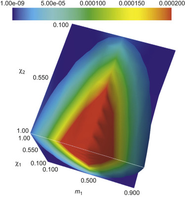 |
| Figure 8.3
Variance of the principal component in
Eq. 8.5
as a function of the black hole spin magnitudes
|
8.8. Conclusion
In this chapter, we have shown that CUDA and GPUs are well suited for the exploration of the binary black hole system parameter space in the post-Newtonian approximation, enabling significant insights into the binary black hole inspiral phase space. In the future, GPU computing and CUDA have the potential to make a significant impact in the quest for direct measurement of gravitational radiation.
References
[1]
B. Abbott,
et al.
,
LIGO: the laser interferometer gravitational-wave observatory (2007)
,
Rep. Prog. Phys.
72
(7
) (2009
)
076901
.
[2]
F. Acernese,
et al.
,
Status of Virgo
,
Class. Quantum Grav.
25
(2008
)
114045
.
[3]
B. Aylott,
et al.
,
Status of NINJA: the numerical INJection analysis project
,
Class. Quantum Grav.
26
(2009
)
114008
.
[4]
B. Aylott,
et al.
,
Testing gravitational-wave searches with numerical relativity waveforms: results from the first Numerical INJection Analysis (NINJA) project
,
Class. Quantum Grav.
26
(2009
)
165008
.
[5]
M. Boyle, A. Buonanno, L.E. Kidder, A.H. Mroue, Y. Pan, H.P. Pfeiffer,
et al.
,
High-accuracy numerical simulation of black-hole binaries: computation of the gravitational-wave energy flux and comparisons with post-Newtonian approximants
,
Phys. Rev.
D78
(2008
)
104020
.
[6]
A. Buonanno, Y. Chen, M. Vallisneri,
Detecting gravitational waves from precessing binaries of spinning compact objects: adiabatic limit
,
Phys. Rev.
D67
(2003
)
104025
.
[7]
A. Buonanno, Y. Chen, M. Vallisneri,
Erratum: detecting gravitational waves from precessing binaries of spinning compact objects: adiabatic limit
,
Phys. Rev.
D74
(2006
)
029905
.
[8]
M. Campanelli, C.O. Lousto, H. Nakano, Y. Zlochower,
Comparison of numerical and post-Newtonian waveforms for generic precessing black-hole binaries
,
Phys. Rev.
D79
(2009
)
084010
.
[9]
S. Kee Chung, L. Wen, D. Blair, K. Cannon, A. Datta,
Application of graphics processing units to search pipeline for gravitational waves from coalescing binaries of compact objects
,
Class. Quantum Grav.
27
(2010
)
135009
.
[10]
J.R. Dormand, P.J. Prince,
A family of embedded Runge-Kutta formulae
,
J. Comput. Appl. Math.
6
(1
) (1980
)
19
–
26
.
[11]
C.R. Galley, F. Herrmann, J. Silberholz, M. Tiglio, G. Guerberoff, Statistical constraints on binary black hole inspiral dynamics Cornell University Library, Preprint arXiv.org, Cornell University Library (2010) arXiv:1005.5560.
[12]
M. Hannam,
Status of black-hole-binary simulations for gravitational-wave detection
,
Class. Quantum Grav.
26
(2009
)
114001
.
[13]
M. Hannam, S. Husa, B. Bruegmann, A. Gopakumar,
Comparison between numerical-relativity and post-Newtonian waveforms from spinning binaries: the orbital hang-up case
,
Phys. Rev.
D78
(2008
)
104007
.
[14]
F. Herrmann, J. Silberholz, M. Bellone, G. Guerberoff, M. Tiglio,
Integrating post-Newtonian equations on graphics processing units
,
Class. Quantum Grav.
27
(2010
)
032001
.
[15]
B. Willke,
GEO600: status and plans
,
Class. Quantum Grav.
24
(2007
)
S389
–
S397
.
[16]
B. Zink, A General Relativistic Evolution Code on CUDA Architectures, Technical Report CCT-TR-2008-1, Louisiana State University, Center for Computation and Technology
http://www.cct.lsu.edu/CCT-TR/CCT-TR-2008-1
, 2008.
..................Content has been hidden....................
You can't read the all page of ebook, please click here login for view all page.