
Chapter 11. Accurate Scanning of Sequence Databases with the Smith-Waterman Algorithm
Łukasz Ligowski, Witold R. Rudnicki, Yongchao Liu and Bertil Schmidt
Because of the advances in high-throughput sequencing technologies, publicly available protein sequence databases continue to grow rapidly. Biologists frequently need to scan these databases to find similar sequences in order to annotate a query sequence of unknown functionality. In this chapter we present how the dynamic programming-based Smith-Waterman (SW) algorithm for protein sequence database scanning can be optimized on GPUs. Starting from a basic CUDA implementation, we discuss several optimization techniques using shared memory, registers, loop unrolling, and CPU/GPU partitioning. The combination of these techniques leads to a fivefold performance improvement on the same hardware. Smith-Waterman is one of the most popular algorithms in bioinformatics, and therefore, the optimization techniques presented in this chapter are beneficial and instructive to researchers in this area.
11.1. Introduction, Problem Statement, and Context
Let us assume that a biologist has just obtained the sequence of a protein that is important for the biological problem under scrutiny. The first question to be asked is whether the function of the protein is already known. This can be answered by aligning this new sequence (query) to the database of all protein sequences with known functionalities to detect similar sequences. Pairwise sequence similarity may be defined by edit distance; that is, the number of edit operations (substitutions, deletions, insertions) required for transforming one sequence into the other
[1]
. Another definition of similarity is based on a so-called substitution matrix and gap penalties. A substitution matrix is a symmetric, pairwise measure of similarity between amino acids (the basic building blocks of proteins)
[2]
. Similar amino acid pairs correspond to positive entries and dissimilar ones to negative entries. The best possible alignment of two sequences is the one with the highest similarity score obtained for any pair of substrings from the two input sequences. The algorithm for finding such a pair of substrings was proposed by Smith and Waterman
[3]
. The Smith-Waterman algorithm is based on dynamic programming (DP). Unfortunately, the algorithm has a quadratic time complexity in terms of the lengths of the two input sequences and is therefore rather slow. Consequently, there has been significant effort to improve the speed of SW for scanning large databases using various techniques, including vectorization on standard multicores
[4]
[5]
and
[6]
, Field Programmable Gate Arrays (FPGAs)
[7]
[8]
[9]
and
[10]
, Cell/BE
[11]
[12]
[13]
and
[14]
and GPUs
[15]
[16]
[17]
[18]
and
[19]
. The goal of this chapter is to show various approaches for implementing the SW algorithm on GPUs using
CUDA and explain various optimization techniques that lead to a fivefold performance improvement of the basic CUDA implementation on the same hardware.
11.2. Core Method
The SW algorithm computes the optimal local pairwise alignment of two given sequences
Q
(query) and
T
(target) of length
 and
and
 using DP with the following recurrence relations:
 where
where
 is a substitution matrix,
 is the gap opening penalty, and
 is the gap extension penalty. The above recurrences are computed for
 and
and
 and are initialized as
 for
for
 . Typical values for the gap penalties would be
 and
and
 . An example of a simple substitution matrix is
 if
if
 and
and
 if
if
 . However, in practice, more complex substitution matrices (such as BLOSUM62
[2]
) that model biochemical properties of amino acids are used.
. However, in practice, more complex substitution matrices (such as BLOSUM62
[2]
) that model biochemical properties of amino acids are used.
The score of the optimal local pairwise alignment is the maximal score in matrix
H
(maxScore
). The actual alignment can be found by a trace-back procedure. However, for SW-based protein sequence database scanning, we just need to compute
maxScore
for each query/database sequence pair. Database sequences are then ranked according to their
maxScore
value and the top hits are displayed to the user. Note that the score-only computation can be done in linear space and does not require storing the full DP matrix.
The described algorithm is embarrassingly parallel because each target/query alignment can be performed independently. GPU ports of SW are specifically designed to improve the speed of scanning of large databases. The main problem during the design of a CUDA algorithm is to find the most efficient use of various types of memory as well as registers to achieve highest possible performance.
11.3. CUDA implementation of the SW algorithm for identification of homologous proteins
The SW algorithm can be used for two applications:
1. Computing an optimal pairwise alignment
2. Scanning a database with a query sequence
The first application usually takes a negligible amount of time even for very long sequences. The second application, however, is highly time-consuming owing to the enormous growth of sequence databases. Acceleration of this task can be achieved in two ways: either by improving the speed of individual alignment or by computing a large number of alignments in parallel. In this chapter we present the design of a massively parallel SW algorithm for database scanning on GPUs.
Our design concentrates on the SW algorithm for protein sequences. Three examples of protein databases that scientists routinely scan are:
• The NR database from NCBI. NR currently consists of 10.8 million sequences comprising 3.7 billion residues;
• The SwissProt database from SIB and EBI. SwissProt currently contains 516,000 sequences comprising 182 million residues; and
• The ASTRAL.SCOP database contains sequences of protein domains with known 3-D structures obtained from the Protein Data Bank. It currently contains 16.7 thousand sequences comprising 2.9 million residues.
The average sequence length in NR and SwissProt is around 350 residues and the longest sequence length is around 35,000 residues.
Assume that the length of the query length is between 100 and 1000 residues. Then the total number of DP matrix cells to be computed is in the range 370–3700G for NR, 18–180G for SwissProt, and 0.29–2.9G for ASTRAL.SCOP. Performance of the SW algorithm is commonly measured in cell updates per second (CUPS). A nonvectorized and single-threaded C implementation of SW achieves a performance of around 0.1 GCUPS (giga CUPS) on a standard CPU. This would translate in a scanning time of up to 10 hours for the NR database. In the following section, we will show how CUDA and a GPU can be used to significantly improve this runtime.
Our approach takes advantage of inherent data parallelism: each database sequence can be aligned independently. Therefore, each CUDA thread can separately perform a different pairwise query-database alignment. Overall scanning speed will then depend on clever organization and implementation of memory access and computation.
In order to achieve good load balancing, database sequences are sorted with respect to their length in decreasing order as a preprocessing step. This guarantees that all threads within the same thread block can work on sequences with similar lengths. We load these sequences into the CUDA shared memory for fast high-bandwidth access. Because of the limited shared memory capacity, special care might be necessary for very long sequences. In our description we will initially skip those cases, assuming that they are processed by the standard CPU algorithm. Later on we will return to this issue and propose a method that can take care of sequences of arbitrary length.
After sorting the database, we split it into chunks consisting of sequences with similar length. Each chunk can be processed by a single kernel. Naturally, the number of sequences in the single chunk should be equal to the optimal number of threads running concurrently on the GPU. For example, let us assume that we use a GTX 280 card with 30 multiprocessors and that the optimal number of threads is 256 per multiprocessor. Then each database chunk should consist of 7680 sequences. With 10.8 million sequences in the NR database, this provides about 1400 chunks, and 1400 kernels are required to process the entire database. We further assume that the card has sufficient memory to hold the entire database.
11.3.1. Version 1 — Simple Implementation of the SW Algorithm on GPU Using CUDA
We fill the DP matrices vertically, in column-major order. The substitution matrix is located in the shared memory; all other matrices are located in the global memory. Other variables are located in registers. We start with initialization of the first row and first column with zeros.
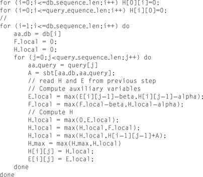 |
One should notice that formally in the SW algorithm
E
,
F
, and
H
are two-dimensional arrays, but the algorithm utilizes only a single column of
E
and
H
and a single value of
F
. This is particularly important for an SW CUDA implementation because the quadratic space required by the two-dimensional matrices
E
,
F
, and
H
would easily exhaust the available global memory. In the pseudo code above we denote
E
and
H
by two-dimensional arrays for clarity; however, in the real code only one-dimensional matrices are used.
It is useful to make a simple analysis of the algorithm to identify bottlenecks. To this end one counts useful instructions performed in the kernel — arithmetic operations, operations on the memory, etc. The maximal theoretical performance of the code is the number of instructions which can be executed by all processors of GPU divided by number of instructions required by algorithm. The real world performance is always lower, due to multiple factors, including memory bandwidth and latency, memory access conflicts, shuffling of data between registers, synchronisation, etc. Very often the memory bandwidth, and not the operation count, is limiting the performance of the algorithm. Therefore, one should always check whether memory bandwidth is sufficient to deliver all data required by the algorithm.
In the preceding pseudo-code operation count in the inner loop is following:
max
– 6,
add
– 9,
shared
load
/
store
2,
global
load
/
store
4, 21 instructions in total, assuming that processor does not need any auxiliary instructions.
The theoretical peak memory bandwidth of a single GPU on a Tesla C1070 board is 102 GB/s. Realistically, one can achieve at most about 70% efficiency of bandwidth usage on applications as simple as copying data; more complicated tasks yield even less bandwidth efficiency. Therefore, taking into account the number of memory operations required by the algorithm, the bandwidth limits the performance of the simple implementation to about 4.5 GCUPS. On the other hand, the theoretical maximal performance of the code,
assuming ideal timing of instructions and assuming that the executable code, assuming ideal timing of instructions and assuming that the executable code contains a minimal number of instructions, is roughly 14.8 GCUPS ( GHz/21 instructions). The implementation is therefore memory bound.
The practical implementation based on this algorithm achieves about 1.7 GCUPS on a Tesla C1070 board. The code of the kernel executing the simple implementation of the SW algorithm in CUDA is shown in
Figure 11.1
.
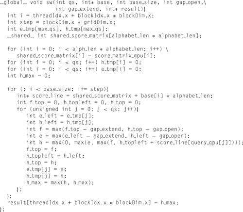 |
| Figure 11.1
The code for the kernel using a straightforward port of the SW algorithm to the GPU.
|
The preceding analysis shows that the optimization of the memory usage is the most effective method for improved performance. A simple way to reduce the amount of data to be accessed from the global memory is to use short integers to represent values of the matrices
E
,
F
, and
H
. This approach halves the number of transactions with the global memory at the price of increased operation count (for reading/storing two short integers in a 32-bit word). After this modification the operation count therefore increases to 25. Thus, the performance limit that is due to operation count decreases to 12.5 GCUPS, whereas the performance limit that is due to memory bandwidth increases to about 9 GCUPS,
which is still not satisfactory. A better approach is redesigning of the code to take advantage of fast shared memory.
11.3.2. Version 2 — Shared Memory Implementation
The shared memory implementation is based on the following idea. The DP matrix is processed in the vertical stripes, parallel to the query. The innermost loop is processing a short column parallel to the query (see
Figure 11.2
). Global memory is accessed only upon entering and exiting this loop. On entrance, the initialization requires reading the relevant values of
H
and
F
from global memory, and on exit, the same variables are stored in the global memory for initialization of the subsequent stripe. All matrices are located either in global memory (suffix Global) or in shared memory (suffix Shared). Other variables are located in registers. Pseudo code for this algorithm is presented below.
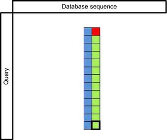 |
| Figure 11.2
An illustration of the use of shared memory. Each thread sequentially computes
|
 |
 |
In the pseudo code above the operation count is as follows:
• main loop per 14 steps:
• load/store from global memory: 4 (2 if H and F are represented by short int)
• load/store from shared memory: 2 (1 if H and F are represented by short int)
• per single step
• load/store from shared memory 4
• add: 4
• max: 6
• TOTAL 14
• total per 14 steps
• load/store from global memory: 4 (2)
• load/store from shared memory: 58 (57)
• add: 56
• max: 84
• TOTAL: 202 (199)
The theoretical performance limit resulting from the instruction count is
 GCUPS. The performance limit that is due to bandwidth is 102 GBs per second/16 bytes per 14 cell
 GCUPS. We can see that by using shared memory, we were able to reduce both the number of instructions and usage of global memory. As a result we obtain much higher theoretical bounds on performance. One should note, however, that the limit that is due to memory bandwidth is now higher than the limit that is due to operation count; that is, the algorithm is bound by the amount of instructions that can be issued by processor, not by the memory. The actual performance of the code is 11 GCUPS on a Tesla C1070 board. The computational kernel is displayed in
Figure 11.3
.
GCUPS. We can see that by using shared memory, we were able to reduce both the number of instructions and usage of global memory. As a result we obtain much higher theoretical bounds on performance. One should note, however, that the limit that is due to memory bandwidth is now higher than the limit that is due to operation count; that is, the algorithm is bound by the amount of instructions that can be issued by processor, not by the memory. The actual performance of the code is 11 GCUPS on a Tesla C1070 board. The computational kernel is displayed in
Figure 11.3
.
 |
| Figure 11.3
The code of the kernel utilizing shared memory.
|
Some additional optimizations are still possible. Load/store operations on shared memory are more than one order of magnitude faster than those on global memory. However, access to the shared memory still requires issuing load/store instructions and can possibly generate access conflicts. Some of the load/store operations can be avoided by explicit loop unrolling. The previous implementation is therefore modified in the following way. The DP matrix is still partitioned in horizontal stripes, but within the innermost loop, we process a rectangular tile of cells. The tile consists of
 cells. The access to the shared memory is performed only for the first (reading) and last (writing) column of the tile. This allows for reducing the number of operations per cell from 14 to 12.
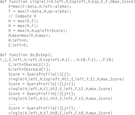
We start by defining the hierarchical set of functions performing computations on different scales of the dynamic programming matrix:
•
single()
— performs an update for a single cell
•
do_8step()
— performs an update for eight adjacent cells (segment) in a single row of the matrix
•
strip_update()
— performs an update for a strip 14 cells high for an entire database sequence length
•
read_helper_data()
— reads data from global memory; this is an auxiliary function reading data required in
strip_update()
•
write_helper_data()
— writes processed variables to global memory; this is an auxiliary function which writes data to global memory
•
DO_STEP(x)
— actually it is a macro, useful to unroll the loop over rows of the tile without actually writing all code manually. The macro is expanded to the
do_8step()
function.
All variables are accessed by reference and therefore their modifications are nonlocal.
 |
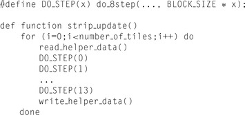 |
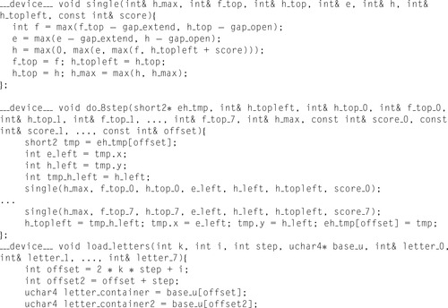
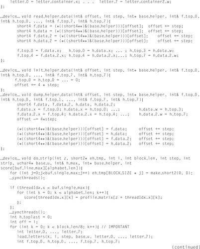
The previously described implementation enables us to reduce the number of operations per cell update to 12. The theoretical performance limit therefore increases to 26 GCUPS. The CUDA program based on this idea achieves 17 GCUPS on a single GPU of a Tesla S1070. One should note, however, that while the theoretical performance limit increased from 21.6 to 26 GCUPS (20%), the performance of the actual code increased by 55% (from 11 to 17 GCUPS) and reached 65% of the theoretical limit. The essential fragments of this kernel are displayed in
Figure 11.4
. One may note that the volume of the code is increased significantly, despite our use of macros for reduction of most repetitive parts. In the actual implementation the additional functions are introduced for the first and last strip.
 |
 |
 |
 |
 |
| Figure 11.4
Listing of the optimized kernel. Repetitive parts of the code replaced by “…”.
|
Initially, we left the problem of long sequences for later. Now, when the code of the basic kernel has been optimized to the last instruction, it is time to handle this problem as well. Initially, we assumed that all sequences processed by a single kernel have similar length, and therefore all threads within all blocks process (almost) identical matrices. When sequence databases are being processed, this is true most of the time, but not all the time. The distribution of the sequence lengths in the SwissProt database has a broad maximum for sequence lengths in the range between 100 and 250. There are about 1000 different sequences at each length in this range.
Then the the number of sequences at given length decreases gradually. This is a distribution with a long thin tail, with longest sequence having over 35000 residues. Unfortunately, one cannot simply ignore these very long sequences.
A sequence block accommodating the longest sequence would take 192 MB, which can be compared with just 182 MB of the entire database. Most of this block would be empty, and the entire kernel performing computations on such a block would wait idling for the single thread performing alignment of the longest sequence. Certainly, it doesn't make sense to put much effort in optimization of the kernels and leave such nonoptimal design.
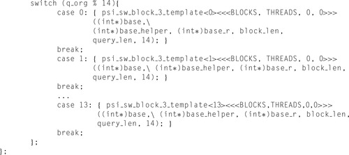
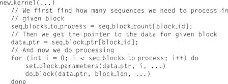
There are two possible solutions for this problem. One is a modification of the GPU kernel to accommodate long sequences. There are many possible ways to modify the kernel. The easiest one is quite simple. Instead of aligning sequences within a whole kernel, we can align sequences only within blocks (or even individual warps within the block). The corresponding kernel may process several sequence blocks within each thread block. The sequence blocks processed by a single-thread block are selected in such a way that the sum of their sizes is similar for all thread blocks within the kernel. In particular, the longest sequence block processed by the first kernel will have a length of about 35,000 residues and will be processed by a single block of threads. The remaining thread blocks process multiple sequence blocks where the sum of the lengths of these blocks will be close to 35,000. In particular, with such kernels the entire SwissProt database can be processed by a single kernel.
The following pseudo code illustrates this kernel. We define a new function,
do_sequence_block
— this function is equivalent to the old kernel. The
new_kernel
function performs computations for several sequence blocks at once.
 |
This solution will work best for large databases, but it will not scale well for smaller ones. Another option is to develop a version of the code in which multiple threads would work on a single sequence, taking advantage of the independence of cells located on the antidiagonal. This solution introduces overhead because some threads must wait for several cell update cycles, until all threads processing higher rows are initialized, but fortunately, this overhead is relatively small for long sequences. One would then call two versions of kernels to process a database containing very long sequences. The kernel with a single thread per sequence would be used for the bulk of the database, whereas the kernel with block per sequence would be used to handle long sequences.
The second method to optimize the kernel for long sequences is radical and simple. One should simply avoid processing these sequences on a GPU in the first place. Instead of developing a more complicated kernel for handling long sequences, one could apply a CPU version of the algorithm running on a CPU for this task. In this way the CPU could be used in parallel to the GPU, instead of sitting idle and waiting until the GPU finishes the task.
11.4. Discussion
Because of the importance of SW in bioinformatics, there have been several attempts to improve its performance using a variety of parallel architectures. The highest performance of the multithreaded SSE2-vectorized CPU version
[6]
is about 15 GCUPS on a modern quad-core CPU
[17]
. This is similar to the performance of the best optimized version of the algorithm described here. Nevertheless, there are some significant disadvantages of the vectorized CPU version. First, its performance drops significantly for short sequences. Second, its performance drops when aligning a query to a large number of similar sequences. Third, its performance is sensitive to the utilized scoring system (i.e., gap penalties and a substitution matrix). In all these situations the GPU algorithm works perfectly well with only minor performance variations.
Even though the optimal alignment scores of the SW algorithm can be used to detect related sequences, the scores are biased by sequence length and composition. The Z-value
[20]
has been proposed to estimate the statistical significance of these scores. However, the computation of Z-value requires the calculation of a large set of pairwise alignments between random permutations of the sequences compared — a process that is highly time-consuming. The acceleration of Z-value computation with CUDA is therefore part of our future work.
11.5. Final Evaluation
The algorithms described in this chapter were developed on and optimized for a Tesla C1070 card. The new Fermi architecture of NVIDIA hardware was available for tests after completing the work. We have been able to evaluate performance of the various versions of the algorithm on the GeForce GTX 480 card. Performance in GCUPS is reported in
Table 11.1
.
Version Ia of
Table 11.1
is the implementation with all variables located in the global memory, and Version Ib is the implementation with the similarity matrix located in the shared memory and query in the constant memory. The performance is roughly 2.5 times higher on the Fermi architecture for the optimized version of the code and 4.6 times higher for the simple port. This is probably due to the cache memory introduced by Fermi. One can see that the difference between both variants of the naive port disappeared because the frequently accessed data from global memory resides in cache. A quick estimate shows that both versions achieve 70% of the theoretical performance limit set by the theoretical global memory bandwidth. Apparently, Fermi performs load/store operations within cache memory, and the memory controller transfers data between cache and global memory with maximal practically achievable speed.
On the other hand, speed increase of the optimized versions of the algorithm is more in line with the difference in raw performance between a Tesla C1070 and a GeForce 480 GTX. The conclusion from this little experiment is that the introduction of the new Fermi architecture significantly improved performance of the naive version, which suggests that automatic porting of applications to CUDA will have a better chance of success than for the previous generations of CUDA-enabled chips. Nevertheless, the code optimized by hand still achieves more than a five-fold speedup in comparison with a naive port.
References
[1]
D. Gusfield,
Algorithms on Strings, Trees, and Sequences: Computer Science and Computational Biology
. (1997
)
Cambridge University Press
,
Cambridge, UK
.
[2]
S. Henikoff, J.G. Henikoff,
Amino acid substitution matrices from protein blocks
,
Proc. Natl. Acad. Sci. U.S.A.
89
(1992
)
10915
–
10919
.
[3]
T. Smiths, M. Waterman,
Identification of common molecular subsequences
,
J. Mol. Biol.
147
(1981
)
195
–
197
.
[4]
A. Wozniak,
Using video-oriented instructions to speed up sequence comparison
,
Comput. Appl. Biosci.
13
(1997
)
145
–
150
.
[5]
T. Rognes, E. Seeberg,
Six-fold speed-up of Smith-Waterman sequence database searches using parallel processing on common microprocessors
,
Bioinformatics
16
(8
) (2000
)
699
–
706
.
[6]
M. Farrar,
Striped Smith-Waterman speeds database searches six times over other simd implementations
,
Bioinformatics
23
(2
) (2007
)
156
–
161
.
[7]
S. Dydel, P. Bała,
Large scale protein sequence alignment using FPGA reprogrammable logic devices
,
In:
Field Programmable Logic and Application, Lecture Notes in Computer Science
,
vol. 3204
(2004
), pp.
23
–
32
.
[8]
T. Oliver, B. Schmidt, D. Nathan, R. Clemens, D. Maskell,
Using reconfigurable hardware to accelerate multiple sequence alignment with ClustalW
,
Bioinformatics
21
(16
) (2005
)
3431
–
3432
.
[9]
T. Oliver, B. Schmidt, D.L. Maskell,
Reconfigurable architectures for biosequence database scanning on FPGAs
,
IEEE Trans, Circuits Syst. II
52
(2005
)
851
–
855
.
[10]
T.I. Li, W. Shum, K. Truong,
160-fold acceleration of the Smith-Waterman algorithm using a field programmable gate array (FPGA)
,
BMC Bioinformatics
8
(2007
)
185
.
[11]
M.S. Farrar, Optimizing Smith-Waterman for the Cell broadband engine.
http://sites.google.com/site/farrarmichael/SW-CellBE.pdf
[12]
A. Szalkowski, C. Ledergerber, P. Krahenbuhl, C. Dessimoz,
SWPS3 — fast multi-threaded vectorized Smith-Waterman for IBM Cell/B.E. and x86/SSE2
,
BMC Res.
Notes 1
(2008
)
107
.
[13]
A. Wirawan, C.K. Kwoh, N.T. Hieu, B. Schmidt,
CBESW: sequence alignment on Playstation 3
,
BMC Bioinformatics
9
(2008
)
377
.
[14]
W.R. Rudnicki, A. Jankowski, A. Modzelewski, A. Piotrowski, A. Zadrożny,
The new SIMD implementation of the Smith-Waterman algorithm on Cell microprocessor
,
Fundamenta Informaticae
96
(2009
)
181
–
194
.
[15]
W. Liu, B. Schmidt, G. Voss, W. Muller-Wittig,
Streaming algorithms for biological sequence alignment on GPUs
,
IEEE Trans. Parallel Distrib. Syst.
18
(9
) (2007
)
1270
–
1281
.
[16]
S.A. Manavski, G. Valle,
CUDA compatible GPU cards as efficient hardware accelerators for Smith-Waterman sequence alignment
,
BMC Bioinformatics
9
(Suppl. 2
) (2008
)
S10
.
[17]
Y. Liu, D.L. Maskell, B. Schmidt,
CUDASW++: optimizing Smith-Waterman sequence database searches for CUDA-enabled graphics processing units
,
BMC Res.
Notes 2
(2009
)
73
.
[18]
L. Ligowski, W. Rudnicki,
An efficient implementation of Smith-Waterman algorithm on GPU using CUDA, for massively parallel scanning of sequence databases
,
In:
IEEE International Workshop on High Performance Computational Biology, HiCOMB 2009, Rome, Italy
(May 25, 2009
)
.
[19]
Y. Liu, B. Schmidt, D.L. Maskell,
CUDASW++2.0: enhanced Smith-Waterman protein database search on CUDA-enabled GPUs based on SIMT and virtualized SIMD abstractions
,
BMC Res.
Notes 3
(2010
)
93
.
[20]
J.P. Comet, J.C. Aude, E. Glémet, J.L. Risler, A. Hénaut, P.P. Slonimski,
et al.
,
Significance of Z-value statistics of Smith–Waterman scores for protein alignments
,
Comput. Chem.
23
(3, 4
) (1999
)
317
–
331
.
..................Content has been hidden....................
You can't read the all page of ebook, please click here login for view all page.