
Chapter 20. Multiclass Support Vector Machine
Sergio Herrero-Lopez
In this chapter we present the GPU implementation of the support vector machine (SVM). The SVM is a set of supervised learning methods used for classification and regression. Given a set of training examples, the SVM algorithm builds a model that predicts the class of new unseen examples. This algorithm is considered essential in both machine-learning and data-mining curriculums and is frequently used by practitioners. Besides, its utilization spans to a wide variety of applied research fields such as computer vision, neuroscience, text categorization, and finance. This study shows that the GPU implementation of the dual form of the SVM using the sequential minimal optimization algorithm leads to performance improvements of an order of magnitude in both training and classification. Finally, a technique that coordinates multiple GPUs to solve even larger classification problems is presented at the end of this chapter.
20.1. Introduction, Problem Statement, and Context
The multiclass classification problem based on SVMs is presented as follows: In multiclass classification, given
ln
-dimensional examples and their corresponding labels
 with
with
 and
Y
= {1, …,
M
}, the goal is to construct a classifier
and
Y
= {1, …,
M
}, the goal is to construct a classifier
 that predicts the label
y
∈
Y
of a new unseen example
that predicts the label
y
∈
Y
of a new unseen example
 . The process of designing the classifier
 from a set of training examples is called the
training phase
, while the process of evaluating the generalization performance of the classifier with a separate dataset of testing examples is known as the
testing phase
[1]
.
from a set of training examples is called the
training phase
, while the process of evaluating the generalization performance of the classifier with a separate dataset of testing examples is known as the
testing phase
[1]
.
The success of SVMs solving classification tasks in a wide variety of fields, such as text or image processing and medical informatics, has stimulated practitioners to do research on the execution performance and scalability of the training phase of serial versions of the algorithm. Nevertheless, the training phase of the SVM remains a computationally expensive task, and the training time of a binary problem composed by 100,000 points with hundreds of dimensions can often take on the order of hours of serial execution.
In this chapter, our contribution is twofold: (1) we provide a single-device implementation of a multiclass SVM classifier that reduces the training and testing time of the algorithm an order of magnitude compared with a popular multiclass solver, LIBSVM, while guaranteeing the same accuracy and (2) we provide an adaptation of the cascade SVM algorithm that uses multiple CPU threads to orchestrate multiple GPUs and confront larger-scale classification tasks
[2]
.
A classical method to solve multiclass SVM classification problems is to decompose it into the combination of
N
independent binary SVM classification tasks
[3]
.
20.2.1. Binary SVM
A binary classification task is the one that given
ln
-dimensional examples and their corresponding labels
 with
with
 and
Y
= {−1, 1}, constructs a classifier
and
Y
= {−1, 1}, constructs a classifier
 that predicts the binary label
y
∈ {−1, 1} of a new unseen example
that predicts the binary label
y
∈ {−1, 1} of a new unseen example
 The binary classifier
 is obtained by solving the following regularization problem:
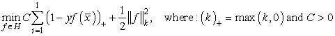 The introduction of slack variables
ξ
i
allows classifying nonseparable data and leads to the
Primal
form:
The introduction of slack variables
ξ
i
allows classifying nonseparable data and leads to the
Primal
form:
 The
Dual
form, which is derived from the Primal, has simpler constraints to be solved:
The
Dual
form, which is derived from the Primal, has simpler constraints to be solved:
 where
where
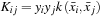 is the kernel function. Common kernel functions are shown in
Table 20.1
. The Dual form (Eq. 20.3
) is a quadratic programming optimization problem, and solving it defines the classification function:
is the kernel function. Common kernel functions are shown in
Table 20.1
. The Dual form (Eq. 20.3
) is a quadratic programming optimization problem, and solving it defines the classification function:
 where
b
is an unregularized bias term. Geometrically, obtaining
where
b
is an unregularized bias term. Geometrically, obtaining
 corresponds to finding the maximum margin hyperplane.
Figure 20.1
(left) illustrates the geometrical interpretation of the binary SVM classifier, and
Figure 20.1
(right) shows the introduction of slack variables when data is not separable. The samples on the margin (α
i
> 0) are called the support vectors (SVs).
corresponds to finding the maximum margin hyperplane.
Figure 20.1
(left) illustrates the geometrical interpretation of the binary SVM classifier, and
Figure 20.1
(right) shows the introduction of slack variables when data is not separable. The samples on the margin (α
i
> 0) are called the support vectors (SVs).
(20.1)
(20.2)
(20.3)
 |
| Figure 20.1
Left: Binary SVM. Right: Binary SVM with nonseparable data.
|
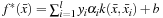
Classical approaches construct the multiclass classifier as the combination of
N
independent binary classification tasks. Binary tasks are defined in the output code matrix
R
of size
M
×
N
, where
M
is the number of classes,
N
is the number of tasks, and
R
ij
∈ {−1, 0, 1}. Each column in matrix
R
represents how multiclass labels are mapped to binary labels for each specific binary task. There are three common types of output codes:
• One-vs-All (OVA):
M
classifiers are needed. For the
 classifier, the positive examples are all the points in class
i
, and the negative samples all the points not in class
i
.
classifier, the positive examples are all the points in class
i
, and the negative samples all the points not in class
i
.
• All-vs-All (AVA):
 classifiers are needed, one classifier to distinguish each pair of classes
i
and
classifiers are needed, one classifier to distinguish each pair of classes
i
and
 is the classifier where class
i
has positive samples and class
j
negative.
is the classifier where class
i
has positive samples and class
j
negative.
• Error-correcting codes: Often error-correcting codes are applied to reconstruct labels from noisy predicted binary labels.
Figure 20.2
(left) illustrates the hyperplanes generated from the resolution of a multiclass SVM problem using AVA output codes, while
Figure 20.2
(right) represents the result using OVA output codes.
 |
| Figure 20.2
Left: All-vs-All (AVA) output code. Right: One-vs-All (OVA) output code.
|
Then each
 is trained separately with
 where
k
= 1 …
N
. The outputs of trained binary classifiers
where
k
= 1 …
N
. The outputs of trained binary classifiers
 along with the output codes
R
yk
and a user-specified loss function
V
are used to calculate the multiclass label that best agrees with the binary predictions:
along with the output codes
R
yk
and a user-specified loss function
V
are used to calculate the multiclass label that best agrees with the binary predictions:
(20.4)
Our approach to solve the multiclass classification problem utilizes the sequential minimal optimization (SMO) algorithm
[4]
. This approach was also successfully used by
[5]
on the implementation of binary classifier for the GPU. Our work takes this previous solution a step further and generalizes the construction of
N
binary classifiers concurrently on the GPU grid. On this section the implementation details of the algorithm are presented.
20.3.1. Sequential Minimal Optimization (SMO)
In order to construct the set of
N
binary classifiers
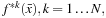 we need to solve
N
quadratic programming (QP) optimization programs on the same set of kernel evaluations
K
, but with different binary labels:
we need to solve
N
quadratic programming (QP) optimization programs on the same set of kernel evaluations
K
, but with different binary labels:
 subject to:
 and
and
 We will use the sequential minimal optimization (SMO) algorithm. SMO solves large-scale QP optimization problems by choosing the smallest optimization problem at every step, which involves only two Lagrange multipliers
 . For two Lagrange multipliers the QP problem can be solved analytically without the need of numerical QP solvers. At each iteration, the two Lagrange multipliers are used to obtain the updated function values
 The SMO algorithm can be directly decomposed into iterations of
Map
and
Reduce
primitives, which have been proven to be very useful extracting parallelism on machine-learning algorithms
[6]
and
[7]
. Different QP programs will have different convergence rates, and the algorithm finishes when the last QP program has converged. Early convergence of some of the QP programs allows binary tasks that are lagging to find a larger number of stream processors available. These are the key steps of the algorithm:
The SMO algorithm can be directly decomposed into iterations of
Map
and
Reduce
primitives, which have been proven to be very useful extracting parallelism on machine-learning algorithms
[6]
and
[7]
. Different QP programs will have different convergence rates, and the algorithm finishes when the last QP program has converged. Early convergence of some of the QP programs allows binary tasks that are lagging to find a larger number of stream processors available. These are the key steps of the algorithm:
(20.5)
1.
Map
: Calculates the new values of the function
 . This step is entirely executed on the device.
2.
Reduce
: The Reduce step combines both host and device segments. These are the substeps that compose the Reduce:
a.
Local Reduce
: Performs reduction operations (max
/
min
and
argmax
/
argmin
) on the device thread blocks.
b.
Global Reduce
: The global reduction is carried out on the host using the output of each device thread block.
c.
Kernel Evaluation
: The calculation of the Lagrange multipliers requires the evaluation of multiple rows of the Gram Matrix
K
. In SVM problems with large numbers of samples and dimensions the storage of matrix
K
in device memory might not be feasible. Consequently, a kernel-caching mechanism was implemented
[8]
. The kernel-cache is managed by the host and stores pointers to the locations of the requested rows of
K
on the device memory.
d.
Update Alphas
: Using the kernel values the Lagrange multipliers are updated on the device so that they are available for the next iteration
 .
.
The core of the algorithm is illustrated in
Figure 20.3
. In the next subsections we include additional details for each step.
 |
| Figure 20.3
SMO algorithm.
|
The Map step updates the values of the classifier function
 based on the variation of the two Lagrange multipliers,
 and the corresponding kernel evaluations:
 with
i
= 1, …,
l
,
k
= 1, …,
N
. The initialization values for the first iteration of the SMO algorithm are
with
i
= 1, …,
l
,
k
= 1, …,
N
. The initialization values for the first iteration of the SMO algorithm are
 .
Figure 20.4
presents the code of the kernel function that executes the Map step. The function takes the following arguments: (1) Input arrays: the function values
d_f
, the binary labels
d_y
,
K
matrix rows
d_k
and the variation of the Lagrange multipliers
d_delta_a
. (2) Indices: the indices of the global locations of the two Lagrange multipliers (d_Iup_global, d_Ilow_global
) and the indices of the cached rows that store the required kernel evaluations (d_Iup_cache, d_Ilow_cache
). (3.) Other parameters: An array pointing to the non-converged binary tasks
d_active
and the number of training samples in the dataset
ntraining
. The Map kernel is launched on a 2-D grid where the blocks along the
x
dimension select specific subsets of the training samples, and the
y
dimension specifies the binary task to work on.
.
Figure 20.4
presents the code of the kernel function that executes the Map step. The function takes the following arguments: (1) Input arrays: the function values
d_f
, the binary labels
d_y
,
K
matrix rows
d_k
and the variation of the Lagrange multipliers
d_delta_a
. (2) Indices: the indices of the global locations of the two Lagrange multipliers (d_Iup_global, d_Ilow_global
) and the indices of the cached rows that store the required kernel evaluations (d_Iup_cache, d_Ilow_cache
). (3.) Other parameters: An array pointing to the non-converged binary tasks
d_active
and the number of training samples in the dataset
ntraining
. The Map kernel is launched on a 2-D grid where the blocks along the
x
dimension select specific subsets of the training samples, and the
y
dimension specifies the binary task to work on.
(20.6)
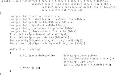 |
| Figure 20.4
The Map step GPU kernel.
|
The Reduce step finds the indices
 and
and
 of the Lagrange multipliers that need to be optimized in each iteration and calculates the new values for
 and
and
 This step interleaves host and device segments. The calculation of the indices is as follows:


(20.7)
(20.8)
The indices are obtained by filtering
Eq. 20.7
and reducing
Eq. 20.8
the
 array. The Local Reduce is carried out on the device and the Global Reduce is performed by the host.
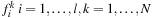
Figure 20.5
shows the Local Reduce kernel function utilized to obtain the
array. The Local Reduce is carried out on the device and the Global Reduce is performed by the host.
Figure 20.5
shows the Local Reduce kernel function utilized to obtain the
 Lagrange multiplier using
min
and
argmin
reductions. The kernel function for the
Lagrange multiplier using
min
and
argmin
reductions. The kernel function for the
 multiplier is analogous, but using
max
and
argmax
operations instead.
multiplier is analogous, but using
max
and
argmax
operations instead.
 |
 |
| Figure 20.5
Kernel function for the reduction of the “Up” Lagrange multiplier.
|
Both kernel functions take similar arguments: (1) Input arrays: the binary labels
d_y
, the current Lagrange multiplier values
d_a
, the function values
d_f
. (2) Output arrays: the value and index of the locally reduced Lagrange multiplier
(d_Bup_local,d_Iup_local)
for the
min
reduction and
(d_Blow_local, d_Ilow_local)
for the
max
reduction. (3) Other parameters: an array pointing to the regularization parameter values
d_c
, an array pointing to the nonconverged binary tasks
d_active
, and the number of training samples in the dataset
ntraining
. The parallel reduction is carried out using a shared memory array,
extern__shared__ float reducearray[]
. The length of this array is specified at kernel launch time. The first half of the array is used to store the reduced values and the second half for the indices. Both reduce kernels are launched on a 2-D grid in which the blocks along the
x
dimension select specific subsets of the training samples, and the
y
dimension specifies the binary task to work on.
After the Local Reduce has been performed in the device, the host finalizes the reduction by finding the global minimum and global maximum with their corresponding indices, which indicate the Lagrange multipliers to be optimized. These two indices per binary task,
 and
and
 also point to the rows of the Gram matrix
K
that will be required in order to calculate the new values of the Lagrange multipliers. A host-controlled LRU (Least Recently Used) cache indicates whether these rows have been previously calculated and are kept in the device memory. A cache hit simply returns the memory location of the required row, whereas a cache miss invokes the CUBLAS
sgemv
routine to calculate the new row and returns its location. In any case, the required 2
N
rows will be in memory before the Lagrange multipliers are updated. The fact that different binary tasks may require the same rows of the Gram matrix
K
increases the cache hit rate.
also point to the rows of the Gram matrix
K
that will be required in order to calculate the new values of the Lagrange multipliers. A host-controlled LRU (Least Recently Used) cache indicates whether these rows have been previously calculated and are kept in the device memory. A cache hit simply returns the memory location of the required row, whereas a cache miss invokes the CUBLAS
sgemv
routine to calculate the new row and returns its location. In any case, the required 2
N
rows will be in memory before the Lagrange multipliers are updated. The fact that different binary tasks may require the same rows of the Gram matrix
K
increases the cache hit rate.
Using the values of these rows of the
K
matrix, we obtain the new values of the Lagrange multipliers:
 where
where
 . Because all the information required to update the Lagrange multipliers resides on the device memory and the Lagrange multipliers themselves will be required by the Map task to be on the device memory as well,
 are calculated on the device using the kernel function in
Figure 20.6
.
are calculated on the device using the kernel function in
Figure 20.6
.
(20.9)
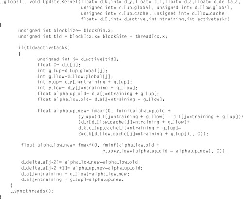 |
| Figure 20.6
Update Alpha kernel function.
|
The Update kernel function takes the following arguments: (1) Input arrays:
K
matrix rows
d_k
, the binary labels
d_y
, the function values
d_f
. (2) Output arrays: the Lagrange multiplier values
d_a
, the variation of the Lagrange multipliers
d_delta_a
. (3) Indices: the indices of the global locations of the two Lagrange multipliers
(d_Iup_global, d_Ilow_global)
and the indices of the cached rows that keep the required kernel evaluations
(d_Iup_cache, d_Ilow_cache)
. (4) Other parameters: an array pointing to the regularization parameter values
d_c
, an array pointing to the nonconverged binary tasks
d_active
, the number of training samples in the dataset
ntraining
and the number of nonconverged binary tasks
activeTasks
. Both reduce kernels are launched on a 2-D grid where the blocks along
the
x
dimension select specific subsets of the training samples, and the
y
dimension specifies the binary task to work on.
Finally, once the new Lagrange multiplier values have been calculated, we check for convergence of the QP program: If
 task
k
has converged, where
τ
is the tolerance parameter. The algorithm finishes when all the
N
tasks have converged.
task
k
has converged, where
τ
is the tolerance parameter. The algorithm finishes when all the
N
tasks have converged.
20.3.4. Testing Phase
In the testing phase, we need to calculate
 for
k
= 1 …
N
and
for
k
= 1 …
N
and
 For each test sample
 it is required to evaluate an entire row
 of the kernel matrix, this row
will be shared by all
N
binary tasks. In order to increase the efficiency of the calculation, we classify as many test samples
of the kernel matrix, this row
will be shared by all
N
binary tasks. In order to increase the efficiency of the calculation, we classify as many test samples
 simultaneously as allowed by the device memory.
We estimate the maximum number
P
of test samples that we can classify at a time based on the available device memory, and we break the test dataset into partitions of
P
samples. For each of these partitions we calculate
 using CUBLAS
sgemm
. Then for each sample
p
= 1 …
P
, we carry out a parallel reduction on the device to calculate
using CUBLAS
sgemm
. Then for each sample
p
= 1 …
P
, we carry out a parallel reduction on the device to calculate
 This step is called
Test Reduce
and is illustrated in
Figure 20.7
. Finally, back in the host, we add the unregularized bias parameter
b
k
to obtain
This step is called
Test Reduce
and is illustrated in
Figure 20.7
. Finally, back in the host, we add the unregularized bias parameter
b
k
to obtain
 and calculate (4).
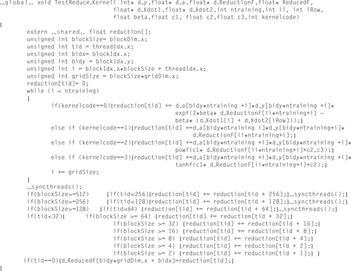 |
| Figure 20.7
Test Reduce kernel function.
|
The Test Reduce kernel function takes the following arguments: (1) Input arrays: the binary labels
d_y
, the Lagrange multiplier values
d_a
, an array with the dot products of the training samples
d_Xdot1
, an array with the dot products of the testing samples
d_Xdot2
, an array with the results of the
sgemm
operation
d_ReductionF
. (2) Output arrays: the array that will store the results of the reduction
d_ReducedF
. (3) Other parameters: the number of training samples in the dataset
ntraining
, the index of the test sample local to the partition being processed
ii
, the index of the test sample global to the test dataset
iRow
, the parameters kernel functions
beta, c1, c2
, and
c3
and the indicator of the kernel function used
kernelcode
. The kernel is launched on a 2-D grid where the blocks along the
x
dimension select specific subsets of the testing samples, and the
y
dimension specifies the binary task to work on.
20.3.5. Size of Device Blocks and Grids
In general, maximum multiprocessor occupancy does not necessarily guarantee best performance. Nevertheless, we chose the number of threads per block and the number of blocks per grid to maximize the device multiprocessor occupancy, but then searched the performance peak experimentally. Fortunately, for the case of multiclass SVMs, maximum occupancy and higher performance resulted to be aligned. Because of the similar nature of the Map, the Local Reduce, and Test Reduce kernel functions, the same block and grid sizes were used in all three cases.
•
Grid size
: Devices with CUDA Compute Capability 1.2 that have eight thread blocks per multiprocessor. Hence, on a device with eight multiprocessors 64 thread blocks can be executed simultaneously. For this reason we set the maximum number of blocks on the
x
dimension of the grid to 64. The
y
dimension of the grid is imposed by the number of nonconverged binary tasks. This arrangement ensures that all the blocks corresponding to the same binary task are being processed simultaneously.
•
Block size
: The register and shared memory usage determine the maximum number of threads per block. The
Map_kernel
uses 11 registers per thread and 92 bytes of shared memory per block. Both
Local_Reduce_KernelMin
and
Local_Reduce_KernelMax
use 13 registers per thread and 1104 bytes of shared memory per block. The
Test_Reduce_kernel
uses 14 registers per thread and 608 bytes of shared memory per block. In all three cases, 100% of multiprocessor occupancy is achieved by setting the maximum number of threads per block to 128.
Large classification problems achieve maximum occupancy by using 128 threads per block and 64 blocks per binary task. This implementation will also work for small classification problems by launching kernel functions with less of blocks and less threads. However, these cases might not result on a 100% of multiprocessor occupancy and consequently would be suboptimal.
The Update kernel function launches one thread per nonconverged binary task on a one-dimensional grid of blocks. The maximum number of threads per block is set to 128. In practice most classification problems involve less than 128 binary tasks; hence, a single block will be launched. This leads to low multiprocessor occupancy, but it is still faster than moving the computation of the Lagrange multiplier update to the host.
20.3.6. Multi-GPU Cascade SVM
Graf
et al.
proposed an algorithm that would allow solving large-scale classification problems on clusters using individual instances of SVMs on a
Cascade
topology
[2]
. The characteristics of different topologies were investigated by Lu
et al
.
[12]
. In both cases, parallelism was achieved by distributing
the SVM problem across multiple machines running single-threaded SVM solvers. In this section, we explain how we adapted the
Cascade SVM
algorithm to run on a multicore and multi-GPU scenario.
In order to orchestrate the operation of multiple devices, a
port-based asynchronous messaging
pattern was used. Typically,
ports
are communication end points associated to a
state
. The posting of a
message
to a port is followed by a predefined
handler
receiving and processing the message based on the actual state. Each port is composed by a queue and a thread pool that manages the messages as they arrive. The existence of this queue makes posting a nonblocking call, letting the sender thread proceed to do other work
[9]
.
In the Multi-GPU Cascade SVM algorithm, each SVM instance is associated to a single device and the state of the SVM is composed by all the variables involved in the training and testing phases. We added a port with the corresponding queue and thread pool on top of the SVM to handle messages asynchronously. Finally, message handlers invoke device kernels based on the SVM state and the message type and its content. In general, thread pools in charge of absorbing the messages accumulated in the queue are composed by multiple threads. Nevertheless, some multiprocessor devices only allow being managed by the same host thread during the entire execution of the program in order to maintain the context between device calls. This is the case for devices with CUDA Compute Capability 1.2; therefore, our thread pools were limited to a single thread, thus guaranteeing that communication with the device would be always performed by the same thread. Latest devices enable concurrent kernel execution to be allowed to increase the number of threads in the thread pool. We call the host thread, the
Master
thread, and the threads assigned to each of the devices,
Slave
threads.
Figure 20.8
illustrates the structure of the port used to invoke SVM functions asynchronously; this is the basic building block of the Cascade SVM.
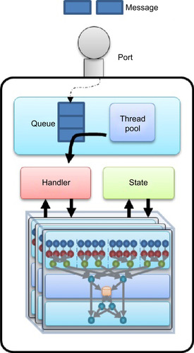 |
| Figure 20.8
GPU SVM instance port.
|
The Multi-GPU Cascade SVM algorithm is composed by a series of
scatter-gather
iterations initiated by the host that work as follows:
1. Given
P
devices the Master thread breaks the training set into
P
subsets and scatters these among available SVM nodes by posting a message containing training samples, training phase parameters, and the response port in which the host will collect all the responses. Each device solves its local multiclass classification problem using the single-device solver described in this chapter. When finished, the obtained SVs are posted back to the response port. The Master thread waits to gather all SVs from
P
devices before proceeding to the next step.
2. The next layer is composed by
P
/2 devices. Each of the devices receives the SVs generated by two devices in the upper level combined pairwise. Each device in this layer solves the local multiclass classification problem using the single-device solver. The values of the Lagrange multipliers are initialized with the SV values of the upper layer. The SVs generated are posted back to the response port of the Master thread. Step 2 is repeated until only a single device is left.
3. The SVs generated by the only device composing the last layer are fed again to the first layer along with shuffled subsets of the non-SV samples. The Lagrange multipliers of the single-device solvers of the first layer are initialized with the SVs provided by the last layer. Convergence is obtained when the set of SVs returned by the last layer remains unchanged. Typically, a single iteration provides comparable accuracy to the single-device solver.
Figure 20.9
illustrates the structure of the Multi-GPU Cascade SVM and its modular composition using multiple instances of the single-device solver.
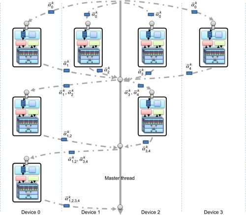 |
| Figure 20.9
Multi-GPU Cascade SVM.
|
Experimental results show that the single-GPU multiclass-SVM solver can reduce the training phase and testing phase time an order of magnitude compared to LIBSVM, a de facto established reference serial implementation for SVM training and classification
[10]
. In addition to increased performance, test results with multiple benchmark datasets demonstrate that the GPU implementation guarantees the same accuracy as LIBSVM. Furthermore, the orchestration of multiple GPUs following the
Cascade SVM
algorithm can introduce an additional order of magnitude of acceleration on top of the already-gained time reduction. In order to provide a representative comparison, special attention was given to use the same configuration parameters for both the GPU and the serial implementation.
– Same kernel types: Radial Basis Function:
– Same regularization parameter C.
– Same stopping criteria.
– Both SMO based.
– Both use One-vs-All (OVA) output codes.
– Same kernel cache size 1GB.
– Both consider I/O an intrinsic part of the classifier.
The performance measurements were carried out using publicly available benchmark datasets. ADULT
[13]
, WEB
[4]
, MNIST
[14]
and USPS
[15]
datasets were used to test the correctness of
single-binary classifications tasks. MNIST and USPS datasets were converted from multiclass to binary problems considering only even versus odd values. Then, MNIST, USPS, SHUTTLE, and LETTER
[16]
datasets were used to analyze the accuracy and performance in multiclass problems. The sizes of these datasets and the parameters used for training are indicated in
Table 20.2
.
20.4.1. GPU SVM Performance
The performance tests measured in this subsection were carried out in a single machine with Intel Core i7 920 @ 2.67GHz and 6GB of RAM running Ubuntu 9.04 (64 bit). The graphics processor model used was a NVIDIA Tesla C1060 with 240 stream processors—each of them with a frequency of 1.3GHz. The card had 4GB of memory and a memory bandwidth of 102GB/s.
Table 20.3
shows the measured training and testing time for both binary and multiclass-SVM problems compared with LIBSVM. All datasets resulted on reductions of the training and testing times. It is observed that the GPU implementation benefited particularly classification problems with the largest numbers of dimensions. MNIST and USPS datasets, which have samples with hundreds of dimensions, resulted in the largest speedup both during the training phase and the testing phase.
The training time was reduced for these datasets in the range of (16x-57x), while the testing time was reduced (13x-112x). Nevertheless, binary and multiclass problems composed by samples with tens of dimensions, such as SHUTTLE or LETTER, obtained a reduced but still respectable acceleration, (3x-25x) for training and (2x-3x) for testing. These results are consistent with the binary SVM in
[5]
.
Table 20.4
shows the comparison of accuracy results for binary and multiclass classification. Results show that classification accuracy in the GPU does as well as the LIBSVM solver. Even if both optimization algorithms run with a tolerance value
τ
= 0.001, there is some variation in the number of support vectors, the value of the offset, and the number of iterations. It is speculated that this difference might be due to the application of second-order heuristics
[11]
or shrinking techniques
[8]
in LIBSVM.
The number of iterations for multiclass problems is not comparable because the GPU solver runs all SMO instances concurrently, whereas LIBSVM does it sequentially.
20.4.2. Multi-GPU Cascade SVM Performance
The execution of the Multi-GPU Cascade SVM algorithm on two layers (four multiprocessor devices) resulted on an additional speedup for the largest and widest datasets. Smaller datasets will not gain additional acceleration, and the parallelization will be affected by the coordination overhead.
The WEB (binary) dataset reduced the SVM training time from 157 s to 106 s (1.48x) resulting on a total acceleration of 22.16x over LIBSVM, while MNIST (OVA 10) reduced the training time from 2067 s to 1180 s (1.75x) resulting on a total of 100.77x over LIBSVM.
20.5. Future Direction
In has been shown in this chapter that a naive implementation of a multiclass classifier based on the SMO algorithm running on a single-multiprocessor device can lead to dataset dependent speedups in the range of 3-57x for training and 3-112x for classification. These results reduced the training time more than an order of magnitude while maintaining accuracy of the classification tasks. Datasets with the largest number of training samples and largest number of dimensions resulted on considerable speedups, while smaller datasets also resulted on a notable acceleration. Furthermore, we have shown that multiple devices can be orchestrated effectively using port-based asynchronous programming in order to further increase the acceleration of the training phase or tackle larger classification problems.
The future direction of this work is threefold: first, the sparse nature of many classification problems requires investigating the effect of the integration of sparse data structures and sparse matrix and vector multiplications on the GPU SVM implementation. Second, it is necessary to extend this GPU SVM implementation in order to be able to learn from data streams. For this purpose it is necessary to revisit the possibilities of exploitation of structural parallelism in online SVM solvers both in the primal
[18]
and dual
[17]
forms. Third, it is necessary to investigate the distribution of online SVM solvers across multiple devices in order to be able scale out the data stream classification problem.
References
[1]
V.N. Vapnik,
The Nature of Statistical Learning Theory (Information Science and Statistics)
. (1999
)
Springer
.
[2]
H.P. Graf, E. Cosatto, L. Bottou, I. Durdanovic, V. Vapnik,
Parallel support vector machines: the cascade svm
,
In:
Advances in Neural Information Processing Systems
,
vol. 17
(2005
), pp.
521
–
528
.
[3]
R. Rifkin, A. Klautau,
In defense of one-vs-all classification
,
J. Mach. Learn. Res.
5
(2004
)
101
–
141
.
[4]
J.C. Platt,
Fast Training of Support Vector Machines Using Sequential Minimal Optimization
. (1999
)
MIT Press
,
Cambridge, MA
.
[5]
B. Catanzaro, N. Sundaram, K. Keutzer,
Fast support vector machine training and classification on graphics processors
,
In:
Proceedings of the 25th International Conference on Machine Learning, Helsinki, Finland, July 5–9, 2008, ICML ’08
,
vol. 307
(2008
)
ACM
,
New York
, pp.
104
–
111
.
[6]
J. Dean, S. Ghemawat,
Mapeduce: simplified data processing on large clusters
,
Commun. ACM
51
(1
) (2008
)
107
–
113
.
[7]
C. Chu, S. Kim, Y.A. Lin, Y.Y. Yu, G. Bradski, A. Ng,
et al.
,
Map-reduce for machine learning on multicore
,
NIPS
19
(2007
)
.
[8]
T. Joachims,
Making Large-Scale Support Vector Machine Learning Practical
. (1999
)
MIT Press
,
Cambridge, MA
.
[9]
D.W. Holmes, J.R. Williams, P. Tilke,
An events based algorithm for distributing concurrent tasks on multi-core architectures
,
Comput. Phys. Commun.
181
(2
) (2010
)
.
[10]
C. Chang, C. Lin, LIBSVM: a library for support vector machines. Software available at
http://www.csie.ntu.edu.tw/~cjlin/libsvm/
, 2001.
[11]
S.S. Keerthi, S.K. Shevade, C. Bhattacharyya, K.R.K. Murthy,
Improvements to platt's SMO algorithm for SVM classifier design
,
Neural Comput.
13
(3
) (2001
)
637
–
649
.
[12]
Y. Lu, V. Roychowdhury, L. Vandenberghe,
Distributed parallel support vector machines in strongly connected networks
,
IEEE Trans. Neural Netw.
19
(7
) (2008
)
1167
–
1178
.
[13]
A. Frank, A. Asuncion, UCI Machine Learning Repository. Irvine, CA, University of California, School of Information and Computer Science.
http://archive.ics.uci.edu/ml
, 2010.
[14]
Y. Lecun, L. Bottou, Y. Bengio, P. Haffner,
Gradient-based learning applied to document recognition
,
Proc. IEEE
86
(11
) (1998
)
2278
–
2324
.
[15]
J. Hull,
A database for handwritten text recognition research
,
IEEE Trans. Patten Anal. Mach. Intell.
16
(5
) (1994
)
550
–
554
.
[16]
C.-W. Hsu, C.-J. Lin,
A comparison of methods for multiclass support vector machines
,
IEEE Trans. Neural Netw.
13
(2
) (2002
)
415
–
425
.
[17]
G. Cauwenberghs, T. Poggio,
Incremental and decremental support vector machine learning
,
NIPS
(2000
)
409
–
415
;
(Online Paper)
.
[18]
Z. Liang, Y. Li,
Incremental support vector machine learning in the primal and applications
,
Neurocomputing
72
(10–12
) (2009
)
;
Lattice Computing and Natural Computing (JCIS 2007) / Neural Networks in Intelligent Systems Designn (ISDA 2007), June 2009
.
..................Content has been hidden....................
You can't read the all page of ebook, please click here login for view all page.