
Chapter 29. Fast Graph Cuts for Computer Vision
P.J. Narayanan, Vibhav Vineet and Timo Stich
In this chapter we present an implementation of Graph Cuts with CUDA C. The computation pattern of this application is iterative with varying workloads and data dependencies between neighbors. We explore techniques to scale workload per iteration and how to parallelize the computation with the nontrivial data dependencies efficiently. This study shows the practical use of these techniques and reports the achieved performance on datasets for binary image segmentation and gives an outlook on how to extend the implementation to solve multilabel problems.
29.1. Introduction, Problem Statement, and Context
The work is done in the context of image segmentation. The task of cutting out arbitrary-shaped objects from images is very common in computer vision and image-processing applications. Graph Cuts have become a powerful and popular approach to solve this problem with minimal user input. The range of applications that can be solved with Graph Cuts also includes stereo vision, image restoration, panorama stitching, and so on
[4]
.
Graph Cuts solve energy minimization problems on integer Markov-Random-Fields (MRF). An MRF is a grid of variables where the solution for a single variable is also dependent on the solution of variables in its neighborhood. For example, in image segmentation the MRF has the shape of the image with a one-to-one correspondence between pixels and variables. The solution assigns to each pixel a label that signals if it belongs to the object to cut out or not. The MRF can be thought of as encoding the increased probability for a pixel to belong to the object if its neighbors belong to the object. By taking the solution of neighboring variables into account, we can significantly improve the results of the segmentation. Unfortunately, this also makes the problem NP-hard in the general case. The best reported serial CPU implementation takes 99 milliseconds on a standard dataset of size 640 × 480 for two labels. Our parallel GPU implementation solves the same problem in 7.5 ms, and hence, makes it possible to get the quality improvement Graph Cuts provided into real-time image-processing applications.
29.2. Core Method
To solve the energy minimization problem, a flow network is constructed that represents the MRF. Finding the maximum flow/minimum cut of the network solves the binary energy minimization
problem over the MRF
[3]
. Our implementation follows the Push-Relabel algorithm introduced by Goldberg and Tarjan
[1]
. The algorithm exhibits good data parallelism and maps well to the CUDA programming model. The computation proceeds by repetitively alternating operations push and relabel on the network until a termination criterion is met. The computations update two properties assigned to each variable of the flow network: excess flow and height. The push operations push excess flow from a variable to its neighbors. The relabel operation updates the height property. The convergence of the computation is sped up in practice by periodically performing a special case of breadth-first search on the network to reset the height property
[2]
.
29.3. Algorithms, Implementations, and Evaluations
Figure 29.1
shows pseudo code for the push and the relabel operations, which are the main parts of the Graph Cut algorithm. Both these operations loop over all variables of the network, but update different properties. First, it should be noted that both operations update only active variables. A variable is active if it has positive excess flow and a height less than infinite. Push transports available excess flow to one or more of eligible neighbors. The operation updates the excess flow and edge capacities, while the height property stays constant. Relabel computes the minimum heights of eligible neighbors and the current height of a variable to update this property. Excess flow and edge capacities stay constant.
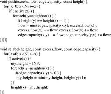 |
| Figure 29.1
Pseudo code for the push and relabel operations.
|
For both operations the results for a single variable are dependent on neighboring data values. This makes their parallelization nontrivial. For now we assume that the computation can be split into quadratic tiles such that there are only data dependencies inside the tiles but none between tiles. There
are different options to achieve this, and we will discuss them in more detail separately. With this tiling, we get a perfect mapping to the CUDA programming model by launching one CUDA block per tile. The threads of one CUDA block cooperate to handle the intratile data dependencies, while there are no interblock dependencies. We set the tile edge length to the GPU warp size of 32. We also assume the neighborhood of the MRF to be the standard 4-neighborhood.
29.3.1. Parallel Push Implementation
For the discussion of the implementation of the push operation, we focus on a single tile and discuss the handling of intertile dependencies at the end of the section. As stated before we launch one CUDA block to handle one tile of the flow network. Although the operation in serial code is simple, we need to be cautious when parallelizing the outer loop because of intratile data dependencies. Looking at the code reveals that a single push from variable
x
to its neighbor
y
updates the excess flow for both
x
and
y
, as well as the edge capacities for
x
−>
y
and
y
<−
x
. First, it is important to note that there will actually be no data access collisions when updating the edge capacities in parallel. The reason for this comes first from the fact that the height property is constant and the if(height(y) == height(x) − 1) condition meaning that flow between neighbors will be pushed only in one direction and never back in one push iteration. Still a one-to-one mapping of variables to threads requires atomic operations to avoid any RAW or WAR hazards when updating the excess flow properties because flow is pushed in multiple directions and can converge into a single variable (see
Figure 29.2
). However, this would not be the optimal choice because atomic operations have reduced achievable peak memory bandwidth and do not support all data types, as, for example, 16-bit integers. A rewrite of the serial push operation, however, shows an alternative to achieve parallel data updates without the need of atomic operations. The idea is to change the order of the loops by looping first over the directions of the neighborhood as follows:
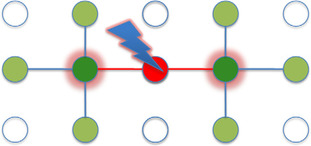 |
| Figure 29.2
Potential data race conditions during updates of the excess flow when flow is pushed from multiple directions into a single variable.
|
void push(excess_flow, edge_capacity, const height) {
foreach(dir=direction) {
for(x=0; x<N; ++x) {
if (active(x)) {
y = neighbor(x,dir);
if(height(y) == height(x) − 1) {
flow = min(edge capacity(x,y), excess flow(x));
edge_capacity(x,y) −= flow; edge_capacity(y,x) += flow
}}}}}
In this version the data dependencies in the inner loop are reduced to one neighbor, the one in the current direction being processed, instead of all neighbors as in the original version. The second idea is to process the variables in the inner loop in the order of the neighbor direction being considered. So for the right neighbor we process like this:
void push_right(row, excess_flow, edge_capacity, const height) {
for(x=row; x<row+Width−1;) {
y = (x+1); // Right neighbor
if (active(x)) {
if(height(y) == height(x) − 1) {
flow = min(edge_capacity(x,y), excess_flow(x));
excess_flow(x) −= flow; excess_flow(y) += flow;
edge_capacity(x,y) −= flow; edge_capacity(y,x) += flow
}}
x = y; // Process in the direction of the neighbor
}}
The code for the other directions is analogous. This rewrite makes it clear that for a single direction first, there are no data dependencies in the directions
orthogonal
to the current neighbor direction. Second, if we further subdivide the processing of a single direction into multiple chunks that are processed in parallel, there is a potential hazard only when accessing the excess flow of the first element of each chunk. This leads to our proposed processing of tiles with one CUDA block. We launch four warps (128 threads) where each thread transports flow over a chunk of 8 pixels per direction, as shown in
Figure 29.3
.
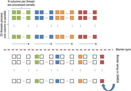 |
| Figure 29.3
In this diagram, 128 threads are pushing flow to the right in a tile of 32 × 32 elements. Each warp of 32 threads transports excess flow in a wavelike pattern. First, each warp transports flow over eight elements in the current direction. After synchronizing, the ninth element in this direction is updated. This avoids data hazards and increases the flow transport distance per operation. The processing is repeated for the other three directions.
|
The update of the neighbor outside of the assigned chunk is done after all threads are synchronized. This step ensures that no data hazard will occur. At this point we also need to discuss how updates to neighbors outside of the current tile are handled. One could argue that using atomic operations just for those is a good choice. However, still atomics are not supported for all data types on all compute devices and also add additional complexity to the code. Instead, we store the updates outside the tiles into a special border array and use a separate kernel to add the border array to the excess flow after each push kernel to avoid data hazards.
So far we have discussed how the parallelization of the push operation is implemented. The next step to achieving good performance is optimizing the memory accesses. During the push operations, the excess flow of the variables is accessed four times for each direction. Hence, we read it once from global memory and process in shared memory to reduce the global memory footprint. Because the height stays constant, the different edge capacities are accessed only once for one push operation, as discussed earlier. Hence, there is no benefit of staging the edge capacities to shared memory, and we read and write to global memory directly. However, during the horizontal waves, the threads of a warp need to access different rows of the edge capacities, resulting in uncoalesced memory accesses. To avoid this we store the horizontal edge capacities in transposed form. This way, accessing the rows in horizontal directions maps to adjacent addresses in global memory, and hence, fully coalesced memory reads and writes.
Finally, the height array must also be accessed read-only during the push operation. Each height value is read multiple times during the push operation, so again, staging to shared memory seems sensible. Unfortunately, the increased shared memory footprint significantly reduces occupancy on pre-Fermi GPUs. Alternatively, because read-only access is sufficient, we can resort to texture fetches on bound linear memory and make use of the texture cache instead. On Fermi GPUs with 48 KB of shared memory per multiprocessor available, the height array is staged to shared memory that results in a slight performance improvement over the texture approach.
29.3.2. Parallel Relabel Implementation
The parallelization of the relabel operation is straightforward. The height properties can all be updated in parallel, and we could launch one thread per variable without having to worry about race conditions. The first idea in improving this naive approach becomes apparent when analyzing the memory accesses. For each thread we check edge capacities to and heights of its neighbors and itself and compute a minimum. Hence, the ratio of memory to arithmetic operations is very high, and the performance of
the kernel is memory bound. To improve, we make use of the fact that a variable
y
is a neighbor in the residual flow network if it is in the 4-neighborhood of
x and if
the edge between
x
and
y
has a capacity greater than 0. If the residual neighbor condition is stored with one bit per neighbor, we can reduce the memory footprint and consequently improve performance.
Although not complex, the implementation of the compression needs some attention to make it right. To enable thread cooperation, we store the compressed residual neighbor condition in shared memory. The smallest memory entities a thread can access are 8-bit words. Hence, we choose to let each thread congest 8-neighbor conditions into one 8-bit word. Another restriction to consider is that on pre-Fermi GPUs, accessing consecutive 8-bit words in shared memory within one warp will cause a four-way bank conflict. This leads us to the computation pattern shown in
Figure 29.4
to achieve a coalesced bank-conflict-free implementation of the compression. Four warps cooperate to compute the result. Each warp processes 32 columns of the edge capacity array, with each thread reading eight rows to build the compressed 8-bit word. The 8-bit words are then scattered into shared memory with a stride of 4 bytes, so bank conflicts are avoided. After the four warps are synchronized, four adjacent 8-bit words computed by the different warps represent 32 compressed elements of one full column. The same pattern is repeated for the other three different edge directions. Because the horizontal edge capacities are stored in transposed form, four adjacent 8-bit words will represent one row of the tile.
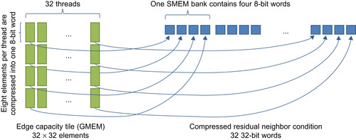 |
| Figure 29.4
Coalesced bank-conflict-free compression of the residual neighbor condition for one direction. Four warps cooperate to compute the result in parallel.
|
29.3.3. Efficient Workload Management
The optimization considerations so far focused on making most efficient use of the GPU and its resources from the implementation point of view. However, these optimizations do not take into account properties of the algorithm and specific workloads. In this section we look at improvements to make the implementation more work efficient as the computation converges toward the final solution.
The key observation is that most of the excess flow that is pushed through the network during processing has reached its final location after a few iterations
[8]
. Still, we continue to process all variables, even if the majority is not active anymore. This step results in very inefficient utilization of the resources from the algorithmic point of view even though the implementation itself is efficient. What we would like to achieve instead, is to process only those variables that are active per the current iteration and skip the ones that are inactive completely. Although implementing such a scaling of the workload per kernel efficiently on the per-variable level is not trivial, there is an easy approach that we can follow instead to achieve a slightly less efficient work scaling. Because we are launching one CUDA block per flow network tile, it is easy to scale the workload on the per-tile level. Instead of launching the CUDA blocks in the full 2-D grid configuration representing the flow network, we build a list of active tiles that are active and launch just enough CUDA blocks to process this list. The active tile list is built using a kernel that stores a 1 for every tile that has any active variables and 0 for others. Compaction is then used to build the list of active tiles. For the push kernel to make use of this, we need to modify it only slightly. First, a new argument, the pointer to the list in GPU memory, is added. Second, we replace the code to compute the 2-D tile offset from the block indices with code to read the assigned list entry and compute the tile offset from the entry instead:
Device
__global__
void push_2D_config(…){
int tile_x = blockIdx.x * 32;
int tile_y = blockIdx.y * 32;
…
Host
…
dim3 grid(Width/32, Height/32);
dim3 block(32,4);
push_2D_config<<<grid,block>>>(…);
…
Device
__global__
void push_list_config(unsigned int* tile_list, …) {
unsigned int tile_id = tile _list[blockIdx.x];
int tile_x = ((tile_id & 0x0ffff0000) >> 16)* 32;
int tile_y = ((tile_id & 0x00000ffff) * 32;
…
Host
…
dim3 grid(tile_list_length);
dim3 block(32,4);
push_list_config<<<grid,block>>>(d_tile_list, …);
…
The final optimization of the basic Graph Cut implementation we consider in this chapter is again motivated from algorithmic observations. First, we point out that the height field is a lower-bound estimate of the geodesic distance of each pixel to the sink in the residual flow network. It has been shown that the more accurate the current estimate, the more effective the push operation will bring the solution toward the final one. Unfortunately, the relabel operation as we implemented it so far can lead to quite poor estimates owing to their local nature. Only direct neighbors are considered, and hence, topological changes can take many kernel invocations to propagate throughout the network. To mitigate this issue, we note that the additional costs of periodically computing the exact distances are more than compensated for with less total iterations and will result in a significant overall speedup. This is also referred to as global relabeling in the literature. In this section we discuss our implementation of global relabeling with CUDA C.
void global_relabel_tile(height) {
done = 0;
while(!done) {
done = 1;
foreach(x of tile) {
my_height = height(x);
foreach(y=neighbor(x)) {
if(edge_capacity(x,y) > 0) {
my_height = min(my_height, height(y)+1);
}
if(height(x) != my_height) {
height(x) = my_height;
done = 0;
}}}}
The correct distances can be computed with a breadth-first search (BFS) of the residual flow network starting from the sink node. The depths in the search tree are the geodesic distances that we are looking for. Discussing a general BFS implementation with CUDA C would fill a separate chapter, but our implementation fortunately has to cover only a special case. The graph we search on is known to have a maximum of four outbound edges per node, and nodes are laid out in a regular grid. The only exception we have to deal with is the sink node that is unbounded and typically has a large number of outbound edges in computer vision problems
[11]
. We handle this exception during the initialization of the search once so that the implementation of the actual search can make use of the regular bounded grid property. During initialization the height is set to 0 if there is an inbound edge from sink (excess
flow<0
), thus taking the first step in the search at this point, and to infinity if a node has no inbound edge from sink (excess
flow>=0
). See
Figure 29.5
.
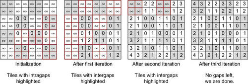 |
| Figure 29.5
Computation pattern of the Global Relabel implementation. Each tile is processed by one CUDA block. Each block updates the heights until there is no change. Tiles at gaps are processed only to achieve efficient workload scaling per iteration.
|
The parallelization of the BFS is then straightforward. We again launch one CUDA block per tile where each block updates the heights of the tile in parallel, as detailed in
Figure 29.5
, until the heights inside the tile do not change anymore. This guarantees that after each kernel execution there will be no gaps in tiles, but only between tiles. A gap in the height field is a height difference between neighbors in the residual graph that is larger than one. In an outer loop we launch this kernel until there are no gaps left and thus the height field contains the solution of the BFS.
Again, the global relabeling implementation can be optimized by applying the strategies from optimizing the push operation. Most obvious, because heights are updated multiple times during operation, it is again beneficial to stage the height tile into shared memory to reduce the traffic to global memory.
Also, instead of launching one thread per variable of the tile, we use the same wave processing that we introduced with the push kernel. This time we don't use it to avoid hazards, but to benefit from its balancing of directed serial updates, which increase information propagation speed throughout the tile, with data parallelism favorably. Finally, we note that launching a 2-D grid of blocks to process all tiles per iteration is similarly work inefficient as it was for the push operation. Changes will proceed as waves through the height field, and only a few tiles will actually change per iteration. So again, we build a list of tiles instead and launch just enough CUDA blocks to process the tiles of the list in each kernel invocation. For the first iteration after initialization, the list contains all tiles that contain height gaps inside the tile itself. Afterward, only the tile boundaries have to be checked for gaps, and only the tiles at intertile height gaps are scheduled for processing in the next iteration (see
Figure 29.5
). The BFS is done when the tile list is empty.
29.4. Final evaluation and validation of results
Table 29.1
summarizes the performance figures for computing the Graph Cut for graphs that represent binary image segmentation problems. The segmentation is based on color models for the foreground and background and also take the image gradients into account. The models are initialized by user input
[12]
as shown in
Figure 29.6
. For the presented figures we did not include the time to compute the data and neighborhood terms. We also compare this performance with that of a CPU implementation that is a different, serial algorithm to compute Graph Cuts
[11]
. Because Graph Cuts find the global optimal solution, the final results are the same.
1
The comparison with the CPU results was also used to verify correctness of our implementation. The average speedup over the test set of an NVIDIA GTX470 in comparison with an Intel Core2 @ 3GHz is 12
x
, varying from 4
x
to 30
x
.
1
For some datasets there exist multiple solutions with the same total global minimal energy (e.g., the Sponge dataset). Graph Cuts return only one of the possibly multiple solutions to a given optimization problem. Hence, we compare the energy of the GPU and the CPU results rather than the two results pixel by pixel.
 |
| Figure 29.6
Example application of Graph Cuts. Left: Flower image from the Middlebury dataset with user input overlaid. Right: Binary image segmentation solution computed with Graph Cuts.
|
Many problems in computer vision can be modeled as the problem to assign a label from a set of labels to each pixel. Examples include stereo correspondence, image restoration, and so on. The labels partition the image into multiple, disjoint sets of pixels. Assigning multiple labels can be mapped to a general multiway cut operation on the graph. Unfortunately, the globally optimal multiway cuts problem is
NP-hard. However, there are algorithms of polynomial complexity that find a local minima solution. One such algorithm is alpha expansion
[10]
, which proceeds in cycles and iterations, each of which involves solving a binary label assignment problem.
Alpha-Expansion Method
The alpha-expansion algorithm is described in this section. The outer loop (steps 2 to 10) forms a cycle, which consists of multiple iterations (steps 3 to 6):
1
Initialize the MRF with an arbitrary labeling
f
.
2
for
each label
alpha
〉 ← L {
3
4
Construct the graph on the current labeling and the label
alpha
.
5
Perform graph cuts to separate vertices of the graph into two disjoint sets.
6
Assign label
alpha
to each pixel in the source set to get the current configuration
f
′.
7
Calculate the energy value
E
(f
′) of the current configuration
f
′.
8
}
9
if
E
(f
′) <
ψ E
(f
) {
10
goto
2
11
}
12
return
f
′;
The algorithm starts from an initial random labeling with each pixel in the image getting a random label from the label set. Iteration alpha (between 1 and L) decides if a pixel gets the label
alpha
or not. This is formulated as a two-level graph cut in which all pixels with a label other than
alpha
participate. After each iteration, each variable retains its current label or takes the label
alpha
. Once all
L
labels are cycled through, the energy of the current configuration is evaluated. This cycle is repeated until no further decrease in energy values is possible.
Step 4 of the algorithm involves a binary graph cut, which can use the parallel GPU implementation described earlier. There are two formulations of the graph for this step. Boykov's formulation
[10]
introduces auxiliary variables, which disturbs the grid structure of the graph. We use Kolmogorov's formulation
[12]
, which maintains the grid structure, but has an additional flag bit for each node to indicate if it takes part in a particular graph cuts step or not.
Incremental Alpha Expansion
Energy minimization algorithms converge faster if the starting point is close to the minima. Intelligent initialization can have a huge impact on the computation time. Reusing the flow as in Kohli and Torr
[6]
is one of the successful methods to initialize better. Alahari
et al
.
[5]
extend this concept to multilabel problems and Vineet and Narayanan
[9]
present a way to exploit relationships within cycles and across cycles in incremental alpha expansion. The final graph of the push-relabel method and the final residual graph of the Ford-Fulkerson method are the same. Each graph is reparametrized based on the final graph of the previous iteration or cycle, as shown in
Figure 29.7
. This incurs additional memory requirements to store
L
graphs, one at the end of each iteration, including their excess flows. Reparametrization is applied to the stored final excess flow from the previous iteration, based on the difference between the initial graphs of the iterations.
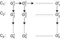 |
| Figure 29.7
Incremental alpha expansion. Arrows indicate the direction of recycling and reparameterization of graphs.
|
Incremental alpha expansion on the GPU results in an average speedup of 5–6 times compared with conducting alpha expansion on the CPU. For more details we refer the interested reader to
[9]
.
[1]
A.V. Goldberg, R.E. Tarjan,
A new approach to the maximum-flow problem
,
J. ACM
35
(4
) (1988
)
921
–
940
.
[2]
B.V. Cherkassky, A.V. Goldberg,
On implementing push-relabel method for the maximum flow problem
,
In:
Proceedings of the 4th International IPCO Conference on Integer Programming and Combinatorial Optimization, Lecture Notes in Computer Science
,
vol. 920
(1995
)
Springer
, pp.
157
–
171
.
[3]
D.M. Greig, B.T. Porteous, A.H. Seheult,
Exact maximum a posteriori estimation for binary images
,
J. R. Stat. Soc. Series B
51
(2
) (1989
)
271
–
279
.
[4]
Middlebury MRF page, Results (plots, images, and code) to accompany
R. Szeliski, R. Zabih, D. Scharstein, O. Veksler, V. Kolmogorov, A. Agarwala,
et al.
,
A comparative study of energy minimization methods for Markov random fields with smoothness-based priors
,
IEEE Trans. Pattern Anal. Mach. Intell. (TPAMI)
30
(6
) (2008
)
1068
–
1080
;
Available from
http://vision.middlebury.edu/MRF
.
[5]
K. Alahari, P. Kohli, P.H.S. Torr,
Reduce, reuse & recycle: efficiently solving multi-label MRFs
,
In:
IEEE Conference on Computer Vision and Pattern Recognition, 23–28 June, 2008
.
Lecture Notes in Computer Science
,
vol. 5996
(2008
)
Springer
,
Anchorage, AK
, pp.
1
–
8
.
[6]
P. Kohli, P.H.S. Tarjan,
Dynamic graph cuts for efficient inference in Markov random fields
,
IEEE Trans. Pattern Anal. Mach. Intell.
29
(12
) (2007
)
2079
–
2088
.
[7]
V. Kolmogorov, R. Zabih,
What energy functions can be minimized via graph cuts?
IEEE Trans. Pattern Anal. Mach. Intell.
26
(2
) (2004
)
147
–
159
.
[8]
V. Vineet, P.J. Narayanan,
CUDA cuts: fast graph cuts on the GPU
,
In:
CVGPU08, CVPR Workshops. IEEE
(2008
), pp.
1
–
8
.
[9]
V. Vineet, P.J. Narayanan,
Solving multilabel MRFs using incremental alpha-expansion on the GPUs
,
In:
Proceedings of the Ninth Asian Conference on Computer Vision (ACCV 09), 23–27 September, 2009
.
Lecture Notes in Computer Science
,
vol. 5996
(2009
)
Springer
,
Xian, China
, pp.
633
–
643
.
[10]
Y. Boykov, O. Veksler, R. Zabih,
Fast approximate energy minimization via graph cuts
,
IEEE Trans. Pattern Anal. Machine Intell.
23
(11
) (2001
)
1222
–
1239
.
[11]
Y. Boykov, V. Tarjan,
An experimental comparison of min-cut/max-flow algorithms for energy minimization in vision
,
IEEE Trans. Pattern Anal. Machine Intell.
26
(9
) (2004
)
;
1124–113
.
[12]
C. Rother, V. Kolmogorov, A. Blake,
GrabCut — interactive foreground extraction using iterated graph cuts
,
ACM Trans. Graph.
23
(2004
)
309
–
314
.
..................Content has been hidden....................
You can't read the all page of ebook, please click here login for view all page.