
Chapter 37. Efficient Automatic Speech Recognition on the GPU
Jike Chong, Ekaterina Gonina and Kurt Keutzer
Automatic speech recognition (ASR) allows multimedia content to be transcribed from acoustic waveforms to word sequences. This technology is emerging as a critical component in data analytics for a wealth of media data that is being generated every day. Commercial usage scenarios are already appearing in industries such as customer service call centers for data analytics where ASR is used to search recorded content, track service quality, and provide early detection of service issues. Fast and efficient ASR enables economic employment of text-based data analytics to multimedia contents. This opens the door to unlimited possible applications such as automatic meeting diarization, news broadcast transcription, and voice-activated multimedia systems in home entertainment systems.
This chapter provides speech recognition application developers with an understanding of specific implementation challenges when working with the speech inference process, weighted finite state transducer (WFST) based methods, and the Viterbi algorithm. It illustrates an efficient reference implementation on the GPU that could be productively customized to meet the needs of specific usage scenarios. To machine learning researchers, this chapter introduces capabilities of the GPU to handle large, irregular graph-based models with millions of states and arcs. Lastly, the chapter provides four generalized solutions for GPU computing researchers and developers to resolve four types of algorithmic challenges encountered during in the implementation of speech recognition on GPUs. These solutions include concepts that are generally useful for creating performance-critical applications on the GPU.
37.1. Introduction, Problem Statement, and Context
It is well-known that automatic speech recognition (ASR) is a challenging application to parallelize
[3]
and
[4]
. Specifically, on the GPU an efficient implementation of ASR involves resolving a series of implementation challenges specific to the data-parallel architecture of the platform. This section introduces the speech application and highlights four of the most important challenges to be resolved when implementing the application on the GPU.
37.1.1. The Speech Recognition Application
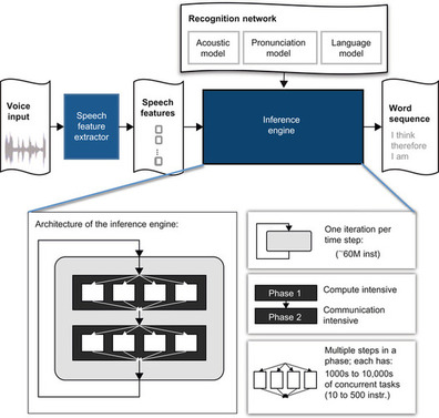
The goal of an automatic speech recognition application is to analyze a human utterance from a sequence of input audio waveforms in order to interpret and distinguish the words and sentences intended by the speaker. Its top-level software architecture is shown in
Figure 37.1
. The inference process uses a
recognition network
, or a
speech model
, which includes three components: an acoustic model, a pronunciation model, and a language model. The acoustic model and language model are trained off-line using powerful statistical learning techniques. The pronunciation model is constructed from a dictionary. The
speech feature extractor
collects feature vectors from input audio waveforms using standard scalable signal processing techniques
[8]
and
[9]
. The
inference engine
traverses the
recognition network
based on the Viterbi search algorithm
[6]
. It infers the most likely word sequence based on the extracted speech features and the recognition network. In a typical recognition process, there are significant parallelism opportunities in concurrently evaluating thousands of alternative interpretations of a speech utterance to find the most likely interpretation
[12]
and
[13]
.
 |
| Figure 37.1
Architecture of a large vocabulary continuous speech recognition application.
|
Algorithmically, ASR is an instance of a machine-learning application where graphical models are used to represent language and acoustic information learned from large sets of training examples. In our implementation, the speech model used is a hidden Markov model (HMM) representing acoustic-, phone-, and word-level transitions, compiled into a unified state machine using WSFT techniques
[5]
. The model is represented as a graph with millions of states and arcs with probabilistic weights. The recognition process performs statistical inference on the HMM using the Viterbi beam search algorithm and iterates through a sequence of extracted input features. Each iteration is one time step and involves two phases of execution. Phase 1 computes the statistical likelihood for a match between an input feature and an element of a database of known phones. This operation is also known as “observation probability computation” and is compute intensive. Phase 2 uses the speech model to infer the most likely sequence seen so far. The computation in Phase 2 involves traversal through a large graph-based model guided by input waveforms. This computation has highly unpredictable control paths and data access patterns and is therefore communication intensive. The output is the most likely word sequence inferred from the input waveform.
37.1.2. The Implementation Challenges
In this chapter, we focus on discussing the four most important challenges when parallelizing the speech recognition inference engine on the GPU. Their solutions are described in
Section 37.2
and elaborated on in
Section 37.3
. The four most important challenges are
1.
Handling irregular graph structures
with data parallel operations;
2.
Eliminating redundant work
when threads are accessing an unpredictable subset of the results based on input;
3.
Conflict-free reduction
in graph traversal to implement the Viterbi beam search algorithm; and
4.
Parallel construction of a global queue
while avoiding sequential bottlenecks when atomically accessing queue-control variables.
Resolving these implementation challenges allows for scalable data-parallel execution of speech recognition applications on the GPU.
37.2. Core Methods
There are efficient solutions for resolving the implementation challenges of speech recognition on the GPU that achieve more than an order of magnitude speedup compared to sequential execution. This chapter identifies and resolves four important bottlenecks in the GPU implementation. The techniques presented here, when used together, are capable of delivering 10.6× speedup for this challenging application when compared to an optimized sequential implementation on the CPU. The four solutions for the implementation challenges are:
1.
Constructing an efficient dynamic vector data structure
to handle irregular graph traversals (Section 37.3.1
)
2.
Implementing an efficient find-unique function
to eliminate redundant work by leveraging the GPU global memory write-conflict-resolution policy (Section 37.3.2
)
3.
Implementing lock-free accesses
of a shared map leveraging advanced GPU atomic operations to enable conflict-free reduction (Section 37.3.3
)
4.
Using hybrid local/global atomic operations and local buffers
for the construction of a global queue to avoid sequential bottlenecks in accessing global queue-control variables (Section 37.3.4
)
Each of the aforementioned solutions is described by first providing the context of the challenge within the automatic speech recognition application. We then proceed by defining the challenge in a generalized problem statement and presenting a solution to the implementation challenge. This allows the solutions to be applied more generally to a variety of machine-learning application areas.
37.3. Algorithms, Implementations, and Evaluations
37.3.1. Constructing an Efficient Dynamic Vector Data Structure to Handle Irregular Graph Traversals
There exists extensive concurrency in the automatic speech recognition application. As shown in
Figure 37.1
, there are 1000s to 10,000s of concurrent tasks that can be executed at the same time in both phases 1 and 2 of the recognition engine.
In a sequential implementation of the speech-inference process, more than 80% of execution time is spent in phase 1. The computation in phase 1 is a
Gaussian mixture model
evaluation to determine the likelihood of an input feature matching specific acoustic symbols in the speech model. The structure of the computation resembles a vector dot product evaluation, where careful structuring of the operand data structures can achieve 16-20x speedup on the GPU. With phase 1 accelerated on the GPU, phase 2 dominates the execution time. Phase 2 performs a complex graph traversal over a large irregular graph with millions of states and arcs. The data-working set is too large to be cached and is determined by input available only at runtime.
Implementing phase 2 on the GPU is challenging
[4]
, as operations on the GPU are most efficient when performed over densely packed vectors of data. Accessing data elements from irregular data structures can cause an order-of-magnitude performance degradation. For this reason, many have attempted to use the CPU for this phase of the algorithm with limited success
[1]
and
[2]
. The suboptimal performance is mainly caused by the significant overhead of communicating intermediate results between phases 1 and 2.
One can implement both phases of the inference engine on the GPU by using a technique for dynamically constructing efficient vector data structures at runtime. As illustrated in
Figure 37.2
, this technique allows the intermediate results to be efficiently handled within the GPU subsystem and eliminates unnecessary data transfers between the CPU and the GPU.
Problem
One often has to operate on large, irregular graph structures with unpredictable data access patterns in machine-learning algorithms. How does one implement the data access patterns efficiently on the GPU?
Solution
The solution involves dynamically constructing an efficient data structure at runtime. Graph algorithms often operate on a subset of states at a time. Let this working set be the “active set.” This active set information is often accessed multiple times within a sequence of algorithmic steps. This is especially true for information about the structure of the graph, such as the set of outgoing arcs emerging from the active states.
 |
| Figure 37.2
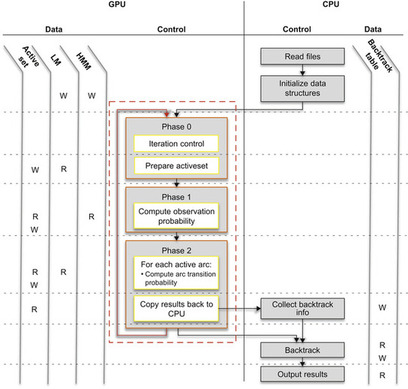
Summary of the data structure access and control flow of the inference engine on many core platforms.
|
Active set information can be dynamically extracted from the overall graph and stored in a contiguous vector for efficient access. The cost of gathering the information is then amortized over multiple uses of the same piece of information.
In automatic speech recognition, this technique is used during aggregation of state and arc properties. As shown in
Figure 37.2
, the “Prepare ActiveSet” step gathers information from the speech model and dynamically populates a set of vectors summarizing the data-working set. This way, the following operations can execute on packed vectors of active states for the rest of the iteration.
The following code segment illustrates the usage of a dynamic runtime buffer:
1
% Gathering operands
2
int
curr_stateID = stateID[i];
3
state_property0[i] = SpeechModel_state_property0[curr_stateID];
4
state_property1[i] = SpeechModel_state_property1[curr_stateID];
5
…
6
% Utilizing gathered operands
7
stepA(stateID, state_property0);
8
stepB(stateID, state_property0, state_property1);
In the preceding code example, there is a
stateID
array that stores a list of the active states. On lines 2 and 3, the properties of an active state
i
are gathered from the graph data structures
SpeechModel_state_property
0 and
SpeechModel_state_property
1 into a consecutive vector of active state properties in the
state_property
0 and
state_property
1 arrays. In subsequent algorithm steps on lines 7 and 8, one can use the dynamically constructed data structure reusing the efficient data layout.
37.3.2. Implementing an Efficient Find-Unique Function to Eliminate Redundant Work
In phase 1 of the inference process, the algorithm computes the likelihood of a match between an input feature vector and elements in a database of known acoustic model units called “triphone states.” In the speech model we used, there is a total of 51,604 unique triphone states making up the acoustic model. On average, only 20% of these triphone states are used for the observation probability computation in one time step.
In a sequential implementation, one can use memoization to avoid redundant work. As the active states are evaluated in phase 1, one can check if a triphone state likelihood has already been computed in the current iteration. If so, the existing result will be used. Otherwise, the triphone state likelihood is computed, and the result is recorded for future reference.
In the parallel implementation, active states are evaluated in parallel and implementing memoization would require extensive synchronization among the parallel tasks.
Table 37.1
shows three approaches that could be used to compute the observation probability in each time step. One approach is to compute the triphone states as they are encountered in the graph traversal process without memoization. This results in a 13 × duplication in the amount of computation required. Even on a GTX280 platform, computing one second of speech would require 1.9 seconds of compute time. A slight improvement to this approach is to compute the observation probability for all triphone states, including the ones that may not be encountered in any particular time step. This results in 4.9× redundancy in the necessary computation, which in turn results in 0.709 second of computation for phase 1 for each second of speech.
The more efficient approach is to remove duplicates in the list of encountered triphone states and compute the observation probabilities for only the unique triphone states encountered during the traversal. This approach requires a fast data-parallel find-unique function.
| *
Real-time factor: the number of seconds required to compute for one second worth of input data
.
| |
| Approaches | Real-Time Factor * |
|---|---|
| 1. Compute only encountered triphone with duplication and no memoization | 1.900 |
| 2. Compute all triphone states once | 0.709 |
| 3. Compute only encountered unique triphone states | 0.146 |
 |
| Figure 37.3
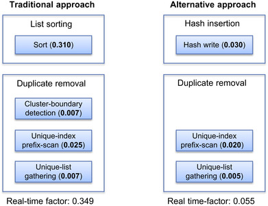
Find unique function approaches.
|
Problem
How does one efficiently find a set of unique elements among tens of thousands of possible elements to eliminate redundant work on the GPU?
Solution
Traditionally, the find-unique function involves a process of “List sorting” and “duplication-removal.” As shown in the left half of
Figure 37.3
, the “sort” step clusters identical elements together, and the “duplication-removal” process keeps one unique element among consecutive identical elements. On a data-parallel platform,
Figure 37.3
illustrates further how the “duplication-removal” process expands into
cluster-boundary identification
,
unique-index prefix-scan
, and
unique list gathering
steps. Specifically, the
cluster-boundary identification
step flags a “1” for the elements that are different than their prior neighbor in the sorted list, and leaves all other positions as “0.” The
unique-index prefix-scan
step computes the index of the cluster-boundary elements in the shortened unique list. The
unique list gathering
step transfers the flagged cluster boundary elements to the unique list. In this sequence of steps, sort is the dominant step with 89% of the execution time of the find-unique function. The sort step alone would take 0.310 seconds to process every second of input data.
An alternative approach is to generate a flag array based on the total number of unique triphone states in a speech model. This is illustrated in the right half of
Figure 37.3
. For the “Hash insertion” process, we leverage the semantics of conflicting writes for non-atomic memory accesses. According to the CUDA Programming Guide
[8]
, at least one conflicting write to a device memory location is guaranteed to succeed. For the purpose of setting flags, the success of any one thread in write conflict situations can achieve the desired result. For the “Duplicate Removal” process, the flag array produced by the
hash write
step can be used directly for
unique-index prefix-scan
and
unique-list gathering
steps. This significantly simplifies the find unique function, providing an efficient way to eliminate redundant work with a small overhead.
37.3.3. Implementing Lock-Free Accesses of a Shared Map to Enable Conflict-Free Reduction
Phase 2 of the automatic speech recognition algorithm performs a parallel graph traversal that is equivalent to a one level expansion during breadth-first search. Starting from a set of current active states, one follows the outgoing arcs to reach the next set of active states. Each state represents an alternative interpretation of the word sequence recognized so far.
The generation of the next set of active states is done in two steps: (1) evaluating the likelihood of a word sequence when an arc is traversed, (2) recording the maximum likelihood of the traversed arc at the destination states (note that maximum likelihood is equal to minimum absolute value in negative log spaces). The first step involves computing the likelihood of particular transitions and is trivially data parallel. The second step involves a reduction over the likelihoods over all transitions ending in a destination state and recording only the transition that produced the most likely word sequence. This is the more challenging step to describe in a data-parallel execution environment.
One can organize the graph traversal in two ways: by
propagation
or by
aggregation
. During the graph traversal process, each arc has a source state and a destination state. Traversal by
propagation
organizes the traversal process at the source state. It evaluates the outgoing arcs of the active states and propagates the result to the destination states. As multiple arcs may be writing their result to the same destination state, this technique requires write conflict-resolution support in the underlying platform. Traversal by
aggregation
organizes the traversal process around the destination state. The destination states update their own information by performing a reduction on the evaluation results of their incoming arcs. This process explicitly manages the potential write conflicts by using additional algorithmic steps so that no write conflict-resolution support is required in the underlying platform.
There is significant overhead in performing the traversal by
aggregation
. Compared with traversal by
propagation
, the process requires three more data-parallel steps to collect destination states, allocate a result buffer for the incoming arcs, evaluate arcs to write to the designated result buffer index, and a final reduction over the destination state. The implementation of each step often requires multiple data-parallel CUDA kernels to eliminate redundant elements and compact lists for more efficient execution.
For traversal by
propagation
, one can implement a direct-mapped table to store the results of the traversal for all states, indexed by the state ID. Conflicting writes to a destination state would have to be resolved by locking the write location, checking if the new result is more likely than the existing result, and selectively writing into the destination state. The approach is illustrated in the following code segment:
1
float
res = compute_result(tid);
2
int
stateID = get_stateID(tid);
3
Lock(stateID);
4
if
(res < stateProbValues[stateID]) {
5
stateProbValues[stateID] = res;
6
}
7
Unlock(stateID);
In the preceding code snippet, each transition evaluation is assigned to a thread. The result of the transition probability is computed by each thread (line 1). Then the
stateID
of the destination state is obtained by each thread (line 2). The
stateProbValues
array provides a lookup table storing the most likely interpretation of the input waveform that ends in a particular stateID. To conditionally update this lookup table, the memory location in the
stateProbValues
array is locked (line 3) to prevent write conflicts when multiple threads access the same state. The location then is updated if the probability computed represents a more likely interpretation of the input waveforms (lines 4–6), which mathematically is a smaller magnitude in log likelihood. Finally, after the update, the memory location for the state is unlocked (line 7).
This approach is not efficient, as recording a result involves two atomic operations guarding a critical section and multiple dependent long-latency memory accesses. In some platforms, because atomic and nonatomic memory accesses may execute out of order, the pseudocode as shown may not even be functionally correct.
Problem
How does one efficiently leverage CUDA capabilities to implement conflict-free reductions when handling large graphs?
Solution
Instead of having a locking/unlocking process for each state update, we take advantage of the
atomicMin()
operation in CUDA and implement a lock-free version of the traversal by
propagation
. The definition of
atomicMin()
is as follows:
1
float
atomicMin(float
* myAddress,
float
newVal);
From the CUDA manual
[7]
, the instruction reads the 32-bit word
oldVal
located at the address
myAddress
in global or shared memory, computes the minimum of
oldVal
and
newVal
, and stores the result back to memory at the same address. These three operations are performed in one atomic transaction. The function returns
oldVal
.
By using the
atomicMin()
instruction, we implement a lock-free shared-array update. Each thread obtains the stateID of the corresponding state and atomically updates the value at that location. The accumulation of the minimum probability is guaranteed by the
atomicMin()
semantics.
2
float
res = compute_result(tid);
3
int
valueAtState = atomicMin(&(destStateProb[stateID]), res);
In the preceding code snippet, each thread computes the likelihood of the transition ending at stateID (line 1) and obtains the stateID of the destination state for its assigned transition (line 2). Then, the destination state transition probability is atomically updated by keeping the smallest magnitude of log-likelihood using the the
atomicMin()
operation. This technique efficiently resolves write conflicts among threads (in the
destStateProb
array on line 3) and thus allows for lock-free updates to a shared array, selecting the minimum value at each array location. The resulting reduction in the write-conflict contention is at least 2× because we have only one atomic operation instead of two locks. The actual performance gain can be much greater because the multiple dependent long-latency accesses in the original critical section between the locking and unlocking processes are also eliminated.
37.3.4. Using Hybrid Local/Global Atomic Operations and Local Buffers for the Construction of a Global Queue
During traversal of the recognition network in the speech-inference engine, one needs to manage a set of active states that represent the most likely interpretation of the input waveform. Algorithmically, this process is done by following arcs from the current set of active states and collecting the set of likely next active states. This process involves two steps: (1) computing the minimum transition probability and (2) collecting all new states encountered into a list.
Section 37.3.3
discusses efficient implementation of the first step on the GPU. If we implement this as a two-step process, after the first step, we would have an array of states where some of the states are marked “active.” The size of this array equals the size of the recognition network, which is on the order of millions of states, and the number of states marked active is on the order of tens of thousands. To efficiently handle graph traversal on the GPU, one needs to gather the set of active states into a dense array to guarantee efficient access of the state data in consequent steps of the traversal process.
One way to gather the active states is to utilize part of the routine described in
Section 37.3.2
, by constructing an array of flags that has a “1” for an active state and a “0” for a nonactive state and then performing a “prefix-scan” and “gather” to reduce the size of the list. However, the prefix-scan operation on such large arrays is expensive, and the number of active states is a less than 1% of the total number of states.
Instead, one can merge the two steps and actively create a global queue of states while performing the write-conflict resolution. Specifically, every time a thread evaluates an arc transition and encounters a new state, it can atomically add the state to the global queue of next active states. The resulting code is as follows:
1
float
res = compute_result(tid);
2
int
stateID = StateID[tid];
3
float
valueAtState = atomicMin(&(destStateProb[stateID]), res);
4
if
(valueAtState == FLT_MAX) {
//
first time seeing the state, push it onto the queue
5
int
head = atomicAdd(&Q_head, 1);
6
myQ[head] = stateID;
7
}
In the code snippet above, each thread evaluates the likelihood of arriving at a state (line 1) and obtains the stateID of the destination state for its assigned transition (line 2). Each entry of the
destStateProb
array is assumed to have been initialized to
FLT
_
MAX
, the largest log-likelihood magnitude (representing the smallest possible likelihood). In line 3, the value in the
destStateProb
array at the
stateID
position is conditionally and atomically updated with the evaluated likelihood. If the thread is the first to encounter the state at
stateID
, the returned value from line 3 would be the initial value of
FLT
_
MAX
. In that case, the new state is atomically added to the queue of destination states. This is done by atomically incrementing the queue pointer variable using the
atomicAdd
operation on the
Q_head
pointer (line 5). The value of the old queue head pointer is returned, and the actual
stateID
can be recorded at the appropriate location (line 6).
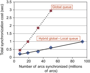
While the merged implementation is an efficient way to avoid instantiating numerous data parallel kernels for collecting active states in the two-step process, there is one sequentializing bottleneck that prevents this implementation from being scalable: when thousands of threads are executing this kernel concurrently, there are thousands of threads atomically updating the
Q_head
variable. As shown in
Figure 37.4
, the synchronization cost of a global queue implementation increases sharply as the number of state transitions evaluated increases.
Problem
How does one efficiently construct a shared global queue?
 |
| Figure 37.4
Comparison of the synchronization cost for global queue and hybrid global and local queue implementations.
|
Solution
In order to resolve the contention on the head pointer, one can use a distributed queue implementation. Each CUDA thread block creates its own local shared queue and populates it every time a thread encounters a new state. After each block constructs its local queue of states, each block then merges its local queue into the global queue. The possible contention on the local queue head pointer is limited to the number of threads in a thread block (usually 64 to 512), and the contention on the global queue head pointer is thus reduced by 64× to 512×, greatly improving performance.
Figure 37.4
shows that the hybrid implementation scales gracefully with an increasing number of arcs. The resulting code is shown below:
2
//
— — — — — — — — — — — — — — — — — — — — — — — — — — — — — — — — — — — — — — — — —
3
extern
__shared__
int
sh_mem[];
// Q size is at most the number of threads
4
int
*myQ = (int
*)sh_mem;
// memory for local Q
5
__shared__
int
myQ_head;
// local Q head ptr
6
__shared__
int
globalQ_index;
// globalQ_index
7
8
if
(threadIdx.x==0) {
9
myQ_head = 0;
10
}
11
__syncthreads();
12
13
int
tid = blockIdx.x*blockDim.x + threadIdx.x;
14
15
if
(tid<nStates) {
16
int
stateID = StateID[tid];
17
float
res = compute_result[tid];
18
19
if
(res > pruneThreshold) {
20
res = FLT_MAX;
21
}
else
{
22
//if res is smaller than prune threshold
23
int
valueAtState = atomicMin(&(destStateProb[stateID]), res);
24
if
(valueAtState == FLT_MAX) {
25
//first time seeing the state, push it onto the local queue
26
int
head = atomicAdd(&myQ_head, 1);
27
myQ[head] = stateID;
28
}
29
}
30
31
// Local Q
–>
Global Q transfer
32
//
— — — — — — — — — — — — — — — — — — — — — — — — — — — — — — — — — — — — — — — — —
33
__syncthreads();
34
35
if
(threadIdx.x==0) {
36
globalQ_index = atomicAdd(stateHeadPtr, myQ_head);
37
}
38
__syncthreads();
39
40
if
(threadIdx.x < myQ_head)
41
destStateQ[ globalQ_index + threadIdx.x] = myQ[threadIdx.x];
42
43
}
// end if (tid<nStates)
In the preceding code snippet, lines 3–6 declare the shared-memory variables: local queue
myQ
and local queue head
myQ_head
index and the head index of the global queue,
globalQ_index
. Thread 0 initializes the local queue head for each block in lines 8–10. The thread ID is computed, and the bounds are checked in lines 13 and 15. Each thread obtains the destination state for its transition and computes the transition probability in lines 16 and 17, respectively. In lines 19–29, the probability for the destination state is updated as described earlier and in
Section 37.3.3
. This time, however, the new states encountered by the threads in each block are stored locally in the local queue (line 26). Once all threads in a thread block have completed their enqueuing operations to the local queue, the thread block adds the content of the local queue to the global queue as a block. Lines 35–37 update the global queue index, and line 41 copies the contents of the local queue to the global queue in parallel.
37.3.5. Performance Analysis
We achieved 10.6× speedup on the GTX280 GPU compared with a highly optimized sequential baseline on a Core i7 CPU. The measurements are taken on the experimental platforms specified in
Table 37.2
. The theoretical upper limit for computation on the platforms are shown as “single-precision giga floating-point operations per second,” or SP GFLOPS/s. The theoretical upper limit for memory bandwidth is shown as GB/s. For the manycore platform setup, we use a Core2 Quad-based host system with 8 GB host memory and a GTX280 graphics card with 1 GB of device memory. The sequential baseline uses one of the cores of a Core i7 CPU.
The speech models are taken from the SRI CALO real-time meeting recognition system
[11]
. The front end uses 13-dimensional perceptual linear prediction (PLP) features with first-, second-, and third-order differences, is vocal-track-length normalized and is projected to 39 dimensions using heteroscedastic linear discriminant analysis (HLDA). The acoustic model is trained on conversational telephone and meeting speech corpora using the discriminative minimum-phone-error (MPE) criterion. The language model is trained on meeting transcripts, conversational telephone speech, and web and broadcast data
[10]
. The acoustic model includes 52,000 triphone states that are clustered into 2613 mixtures of 128 Gaussian components.
The pronunciation model contains 59,000 words with a total of 80,000 pronunciations. We use a small back-off bigram language model with 167,000 bigram transitions. The recognition network is an
H
∘
C
∘
L
∘
G
model compiled using WFST techniques, and contains 4.1 million states and 9.8 million arcs.
The test set consists of excerpts from NIST conference meetings, taken from the “individual head-mounted microphone” condition of the 2007 NIST rich transcription evaluation. The segmented audio files total 44 minutes in length and comprise 10 speakers. For the experiment, we assumed that the feature extraction is performed off-line so that the inference engine can directly access the feature files. The meeting recognition task is very challenging owing to the spontaneous nature of the speech.
1
The ambiguities in the sentences require a larger number of active states to keep track of alternative interpretations that lead to slower recognition speed.
1
A single-pass time-synchronous Viterbi decoder from SRI using lexical tree search achieves 37.9% WER on this test set.
Our recognizer uses an adaptive heuristic to adjust the search beam size based on the number of active states. It controls the number of active states to be below a threshold in order to guarantee that all traversal data fits within a preallocated memory space.
Table 37.3
shows the decoding accuracy, that is, word error rate (WER) with varying thresholds and the corresponding decoding speed on various platforms. The recognition speed is represented by the real-time factor (RTF) that is computed as the total decoding time divided by the duration of the input speech.
As shown in
Table 37.3
, the GPU implementations can achieve significant speedup for the same number of active states. More important, we can improve both the speed and accuracy of the recognition process by using the GPU. For example, compared with the sequential implementation using an average of 3518 active states, the parallel implementation using an average of 32,820 active states can provide a higher recognition accuracy and at the same time see a 3× speedup.
For the next experiment, we choose a beam-width setting that maintains an average of 20,000 active states to analyze the performance implications in detail. The sequential implementation is functionally equivalent with negligible differences in decoding output.
We analyzed the performance of our inference engine implementations on the GTX280 GPU. The sequential baseline is implemented on a single core in a Core i7 quadcore processor. It uses a SIMD-optimized phase 1 routine and non-SIMD graph traversal routine for phase 2. Compared with this highly optimized sequential baseline, we achieve 10.6× speedup on the GTX280.
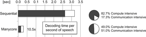
The performance gain is best illustrated in
Figure 37.5
by highlighting the distinction between the compute-intensive phase (black bar) and the communication-intensive phase (white bar). The compute-intensive phase achieves 17.7× speedup on the GPU, while the communication-intensive phase achieves only 3.7× speedup on the GPU.
The speedup numbers indicate that synchronization overhead dominates the runtime as more processors need to be coordinated in the communication-intensive phase. In terms of the ratio between the compute- and communication-intensive phases, the pie charts in
Figure 37.5
show that 82.7% of the time in the sequential implementation is spent in the compute-intensive phase of the application. As we scale to our GPU implementation, the compute-intensive phase becomes proportionally less dominant, taking only 49.0% of the total runtime. The increasing dominance of the communication-intensive phase motivates a detailed examination of parallelization implications in the communication-intensive phases of our inference engine.
 |
| Figure 37.5
Ratio of computation-intensive phase of the algorithm vs. communication-intensive phase of the algorithm.
|
37.4. Conclusion and Future Directions
In this chapter, we demonstrated concrete solutions to mitigate the implementation challenges of an automatic speech recognition application on NVIDIA graphics processing units (GPUs). We described the software architecture of an automatic speech recognition application, posed four of the most important challenges in implementing the application, and resolved the four challenges with the corresponding four solutions on a GPU-based platform. The challenges and solutions are:
1.
Challenge:
Handling irregular graph structures
with data-parallel operations
Solution:
Constructing an efficient dynamic vector data structure
to handle irregular graph traversals
2.
Challenge:
Eliminating redundant work
when threads are accessing an unpredictable subset of data based on input
Solution:
Implementing an efficient find-unique function
by leveraging the GPU global memory write-conflict-resolution policy
3.
Challenge:
Performing conflict-free reduction
in graph traversal to implement the Viterbi beam search algorithm
Solution:
Implementing lock-free accesses
of a shared map leveraging advanced GPU atomic operations with arithmetic operations to enable conflict-free reduction
4.
Challenge:
Parallel construction of a global queue
causes sequential bottlenecks when atomically accessing queue control variables
Solution:
Using hybrid local/global atomic operations and local buffers
for the construction of a global queue to avoid sequential bottlenecks in accessing global queue control variables
Our ongoing research is to incorporate these techniques in an automatic speech recognition inference engine framework that allows application developers to further customize and extend their speech recognizer within an optimized infrastructure for this class of applications.
Figure 37.6
shows a framework with its reference implementation infrastructure at the center and extension points illustrated as notches along the border of the framework. The position of the extension points in the figure signifies the particular algorithm step that an extension point is extending. Each notch can have multiple interchangeable plug-ins. For example, an application developer is able to customize the pruning strategy either with adaptive beam-width thresholds or fixed beam-width thresholds.
 |
| Figure 37.6
An automatic speech recognition inference engine application framework.
|
The extension points listed on the left are execution speed-sensitive extension points that should be customized only by a parallel programing expert. The extension points listed on the right are extension points that provide good execution speed isolation, where any customization affects the speed of only that particular application step.
This kind of application framework provides an optimized infrastructure that incorporates all the techniques discussed in this chapter to allow efficient execution of the speech inference process on the GPU. By allowing flexible customizations of extension points without jeopardizing efficient execution, we believe such frameworks will provide application developers with significant implementation support for constructing efficient and scalable speech recognition applications on the GPU.
References
[1]
P. Cardinal, P. Dumouchel, G. Boulianne, M. Comeau,
GPU accelerated acoustic likelihood computations
,
In:
Proceedings of the 9th Annual Conference of the International Speech Communication Association (Interspeech), 22–26 September 2008
Brisbane, Australia
. (2008
), pp.
964
–
967
.
[2]
P.R. Dixon, T. Oonishi, S. Furui,
Fast acoustic computations using graphics processors
,
In:
Proceedings of IEEE International Conference on Acoustics, Speech, and Signal Processing (ICASSP), 19–24 April 2009
Taipei, Taiwan
. (2009
), pp.
4321
–
4324
.
[3]
A. Janin, Speech recognition on vector architectures, PhD thesis, University of California, Berkeley, CA, 2004.
[4]
A. Lumsdaine, D. Gregor, B. Hendrickson, J. Berry,
Challenges in parallel graph processing
,
Parallel Process. Lett.
17
(1
) (2007
)
5
–
20
.
[5]
M. Mohri, F. Pereira, M. Riley,
Weighted finite state transducers in speech recognition
,
Comput. Speech. Lang.
16
(1
) (2002
)
69
–
88
.
[6]
H. Ney, S. Tarjan,
Dynamic programming search for continuous speech recognition
,
IEEE Signal Process. Mag.
16
(5
) (1999
)
64
–
83
.
[7]
NVIDIA CUDA Programming Guide, Version 2.2
http://developer.download.nvidia.com/compute/cuda/2_2/toolkit/docs/NVIDIA_CUDA_Programming_Guide_2.2.pdf
(2009
)
.
[8]
A. Obukhov, A. Kharlamov,
Discrete cosine transform for 8 × 8 blocks with CUDA, NVIDIA white paper
,
http://developer.download.nvidia.com/compute/cuda/sdk/website/C/src/dct8×8/doc/dct8×8.pdf
(2008
)
.
[9]
V. Podlozhnyuk,
FFT-based 2D convolution, NVIDIA white paper
,
http://developer.download.nvidia.com/compute/cuda/2_2/sdk/website/projects/convolutionFFT2D/doc/convolutionFFT2D.pdf
(2007
)
.
[10]
A. Stolcke, X. Anguera, K. Boakye, O. Cetin, A. Janin, M. Magimai-Doss,
et al.
,
The SRI-ICSI Spring 2007 meeting and lecture recognition system
,
In:
Multimodal Technologies for Perception of Humans, 1 January 2008
,
vol. 4625
(2008
)
Springer
, pp.
450
–
463
.
[11]
G. Tur,
et al.
,
The CALO meeting speech recognition and understanding system
,
In:
Proceedings of the IEEE Spoken Language Technology Workshop, 15–19 December 2008
Goa, India
. (2008
), pp.
69
–
72
.
[12]
J. Chong, Y. Yi, A. Faria, N. Satish, K. Keutzer,
Data-parallel large vocabulary continuous speech recognition on graphics processors
,
In:
Proceedings of the 1st Annual Workshop on Emerging Applications and Many Core Architecture, 21 June 2008
Beijing, China
. (2008
), pp.
23
–
35
.
[13]
K. You, J. Chong, Y. Yi, E. Gonina, C. Hughes, Y. Chen,
et al.
,
Parallel scalability in speech recognition: inference engine in large vocabulary continuous speech recognition
,
IEEE Signal Process. Mag.
26
(2009
)
124
–
135
.
..................Content has been hidden....................
You can't read the all page of ebook, please click here login for view all page.