
The Anatomy of the Airfoil
Abstract
The chapter presents fundamental concepts and theories regarding airfoil lift and drag generation. It begins by presenting crucial definitions for use in airfoil theory. Ranging from the basics of Buckingham’s Π-theory to representation of forces moments to discussion of pressure distribution along the upper and lower surfaces of the airfoil and how it affects the growth of the boundary layer and, eventually, flow separation. Discussion of airfoil stall characteristics and ice-accretion problems are introduced with the basics of airfoil design theory. Then important geometric properties of airfoils are presented to help make the aircraft designer better rounded when comes to identifying various airfoil types, such as NACA airfoils, and understanding of their background. For this purpose, the section introduces a number of airfoils that have gained fame or notoriety in the history of aviation. This is followed by a discussion of the generation of forces and moments on the airfoil and how various outside agents, such as very high airspeeds, high angle-of-attack, deflection of control surfaces, and even surface contamination, affects their aerodynamic properties. Finally, it presents a method to help the designer select the proper airfoil for a new aircraft design.
Keywords
Lift; drag; pitching moment; pressure distribution; flow separation; boundary layer; stall; ice-accretion; NACA 4-digit series; 5-digit series; 1-series; 6-series; 7-series; 8-series; camber; Reynolds number; compressibility; critical Mach number; selection matrix
Outline
8.1.1 The Content of this Chapter
8.1.2 Dimensional Analysis – Buckingham’s Π Theorem
8.1.3 Representation of Forces and Moments
The Smeaton Lift Equation (Obsolete)
8.1.4 Properties of Typical Airfoils
Maximum and Minimum Lift Coefficients, Clmax and Clmin
Angle-of-attack at Zero Lift, αZL
Minimum Drag Coefficient, Cdmin
Lift Coefficient of Minimum Drag, Clmind
8.1.5 The Pressure Coefficient
The Canonical Pressure Coefficient
8.1.6 Chordwise Pressure Distribution
“Conventional” Lift Distribution
8.1.7 Center of Pressure and Aerodynamic Center
Aerodynamic Center and Quarter Chord Moment
Kutta-Joukowski Circulation Theorem
8.1.9 Boundary Layer and Flow Separation
Factors Affecting Laminar Flow
8.1.10 Estimation of Boundary Layer Thickness
8.1.11 Airfoil Stall Characteristics
8.1.12 Analysis of Ice-accretion on Airfoils
8.1.13 Designations of Common Airfoils
8.2 The Geometry of the Airfoil
Thickness, Mean-line and Camber
8.2.2 NACA Four-digit Airfoils
Computation of Airfoil Ordinates
Step 3: Prepare Ordinate Table
Step 5: Compute the y-value for the Mean-line
Step 6: Calculate the Slope of the Mean-line
Step 7: Calculate the Ordinate Rotation Angle
Step 8: Calculate the Upper and Lower Ordinates
Generation of the NACA 4415 – an Example Implementation
8.2.3 NACA Five-digit Airfoils
Computation of Airfoil Ordinates
Step 3: Prepare Ordinate Table
Step 5: Compute the y-value for the Mean-line
Step 6: Calculate the Slope of the Mean-line
Step 7: Calculate the Ordinate Rotation Angle
Step 8: Calculate the Upper and Lower Ordinates
8.2.8 NACA Airfoils in Summary – Pros and Cons and Comparison of Characteristics
8.2.9 Properties of Selected NACA Airfoils
8.3 The Force and Moment Characteristics of the Airfoil
8.3.2 The Two-dimensional Lift Curve
8.3.3 The Maximum Lift Coefficient, Clmax
Maximum Theoretical Lift Coefficient
8.3.4 The effect of Reynolds Number
Compressibility Effect on Lift
Compressibility Effect on Drag
Compressibility Effect on Lift and Drag Exemplified
Compressibility Effect on Pitching Moment
8.3.7 The Critical Mach Number, Mcrit
Step-by-step: Determining Mcrit for a Body
Step 1: Establish the Minimum Pressure Coefficient
Step 2: Select Compressibility Correction Method
Step 3: Solve to Determine Mcrit
8.3.9 The Effect of Addition of a Slot or Slats
8.3.10 The Effect of Deflecting a Flap
8.3.12 The Effect of Deploying a Spoiler
8.3.13 The Effect of Leading Edge Roughness and Surface Smoothness
8.3.14 Drag Models for Airfoils Using Standard Airfoil Data
8.3.15 Airfoil Selection How-to
Impact on Maximum Lift and Stall Handling
Impact on Wing-fuselage Juncture
8.1 Introduction
Any object that moves through a fluid induces a pressure field in its vicinity. The pressure field changes the pressure on its surface and induces a resultant pressure force, R, which acts on the object. Then, we define lift, L, as the component of this force that is normal to the trajectory (or flight path). Similarly, drag, D, is defined as the component of this force tangent to the trajectory. In addition to the pressure force, viscous friction adds to the total drag force. The lift generated by three-dimensional objects is treated in Chapter 9, The anatomy of the wing and drag is treated in Chapter 15, Aircraft drag analysis. However, the purpose of this section is to focus specifically on the important geometric shape used for lifting surfaces: the airfoil.
What sets the airfoil shape apart from other geometry, like, say, the kidney in Figure 8-1, is that its resultant force approaches being normal to the tangent to the trajectory. This results in a lift force component substantially larger than the drag component. Consequently, such geometry generates lift far more effectively than other shapes. The treatment of the airfoil in this section is purely two-dimensional, but this will be expanded to three dimensions in Chapters 9 and 15.

Note that it is a convention in the literature to denote forces and moments for two-dimensional geometry by a lower-case letter but with capitalization when referring to three-dimensional geometry. Thus, lift, drag, and moment for an airfoil would be denoted by l, d, and m, respectively, but using L, D, and M for a three-dimensional wing. The difference between the two, fundamentally, is that a wing has a finite aspect ratio (AR), whereas an airfoil can be considered like a wing of infinite span and, thus, infinite AR. This convention will be adhered to in this text. Consequently, the lift, drag, and moment coefficients for an airfoil are written using lower-case identifiers; Cl, Cd, Cm. Capitalized identifiers are used for 3D wings or an aircraft as a whole: CL, CD, CM.
Many areas of the aircraft design process rely on accurate estimation of these forces and moments. This includes performance analysis, determination of useful load, and structural analysis, to name a few. As has already been alluded to, any competitive aircraft design requires the useful load to be maximized. This implies the empty weight must be minimized and this can only be done if the distribution of pressure loads on the vehicle can be accurately estimated.
When it comes to airplanes, we are mostly interested in bodies whose geometry results in a lift force (L) that is substantially larger than the drag (D). Airfoils are examples of such bodies and, at low angles-of-attack their lift is significantly greater than their drag. As an example, the lift component for modern-day airfoils can be in the excess of 200 times the drag force at some specific orientation in the flow.
8.1.1 The Content of this Chapter
• Section 8.1 presents fundamental concepts and theories regarding airfoil lift and drag generation. It contains very important definitions. Additionally, it introduces how pressure is distributed along the upper and lower surfaces of the airfoil and how it affects the growth of the boundary layer and, eventually, flow separation.
• Section 8.2 defines important geometric properties of airfoils. It also presents information intended to make the aircraft designer better rounded when comes to identifying various airfoil types, such as NACA airfoils, and understanding of their background. For this purpose, the section introduces a number of airfoils that have gained fame or notoriety in the history of aviation.
• Section 8.3 discusses the generation of forces and moments on the airfoil. It details how various outside agents, such as very high airspeeds, high angle-of-attack, deflection of control surfaces, and even contamination, affects their aerodynamic properties. Finally, it presents a method to help the designer select the proper airfoil for a new aircraft design.
8.1.2 Dimensional Analysis – Buckingham’s Π Theorem
Dimensional analysis is a tool used by scientists to confirm derived equations that describe physical phenomena, by enforcing unit consistency. In physics, the fundamental units are mass (m), length (L), time (t), ampère (A), and kelvin (K). All other physical quantities have units that are based on these. As an example, consider pressure, which is defined as force per area. Force is defined as mass times acceleration or m·L/t2. For this reason, it is possible to write pressure as (m·L/t2)/L2 = m/(L·t2). In aerodynamics, forces are denoted as follows:
This matches the units for the force, showing it is dimensionally consistent.
The Buckinham Π theorem, named after Edgar Buckingham (1867–1940), is used to derive the proper form for aerodynamic forces. In general, observation shows that the force generated in a fluid flowing over a body depends on the density of the fluid (more density, larger force), the relative speed of the fluid with respect to the body (more speed, larger force), and the size of the body (larger body, larger force). It is possible to relate these using the following expression:
![]() (8-2)
(8-2)
where
k = unknown constant of proportionality
a, b, c = exponents to be determined
Inserting the dimensions into Equation (8-2) yields:
![]() (8-3)
(8-3)
Simplification on the right side leads to:
![]()
Since the dimensions on the left- and right-hand sides must be consistent, we can determine a, b, and c as follows:

Therefore, we can rewrite Equation (8-3) as follows:
This formulation serves as the basis for all forces and moments used in aerodynamic theory.
8.1.3 Representation of Forces and Moments
The total force (or resultant force) generated by a wing can be found to depend on several parameters: the wing’s geometry, density of air, airspeed, and the angle the chord line of the wing’s airfoils make to the flow of air, the angle-of-attack (from here on also referred to as AOA). While the wing is a three-dimensional, it is usually treated as a set of two two-dimensional geometric features; the airfoil (x-z plane as shown in Figure 8-2) and planform (x-y plane, see Section 9.4, Planform Selection). It was shown by dimensional analysis (i.e. via the Buckingham’s Π theorem) that the equation describing this resultant force, r, is given by:
![]() (8-5)
(8-5)
where
ρ = density of air, in kg/m3 or slugs/ft3
S = reference area, typically wing area, in m2 or ft2
Cr = non-dimensional coefficient that relates AOA to the force
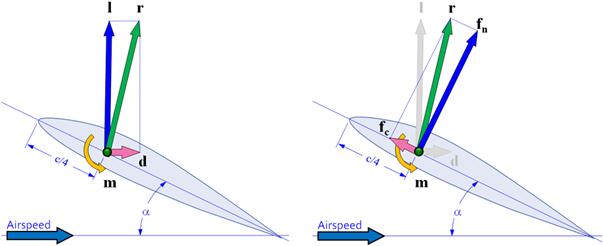
FIGURE 8-2 Forces and moments acting on an airfoil (left) and the definition of normal and chordwise force on an airfoil at a high AOA (right).
Figure 8-2 shows that the lift (force normal to the airspeed), drag (force parallel to the airspeed), and pitching moment (which all are assumed to act at the quarter chord) can be defined as follows:
 (8-6)
(8-6)
Lift and drag are less important to the structural engineer than the normal and chordwise forces, fn and fc, respectively (see Figure 8-2). The normal force is perpendicular (as the name implies) to the wing plane (the hypothetical plane formed by the span- and chordwise vectors) and generates the bending moment. The chordwise force, on the other hand, is parallel to the chord plane. At low angles-of-attack the magnitude of fc is close to the drag force and points toward the trailing edge of the airfoil. However, at high angles-of-attack fc actually points forward, toward the leading edge. The effect tends to move the wing in a forward direction! This effect must be taken into account in structural analysis as it places the aft spar attachment in tension, whereas at low angles-of-attack it places the aft attachment in compression. Figure 8-2 shows that the normal and chordwise forces can be defined as follows:
![]() (8-7)
(8-7)
For three-dimensional objects such as aircraft, the representation of forces and moments that correspond to Equation (8-6) is given by:
 (8-8)
(8-8)
where L, D, M refer to the three-dimensional lift, drag, and pitching moment, respectively. Thus, CL is the three-dimensional lift coefficient, CD the drag coefficient, and CM the pitching moment coefficient of the complete aircraft. These will be treated in more detail in Chapters 9, 11, and 15. CMGC is the wing’s mean geometric chord and S is the reference wing area. Both are presented in detail in Chapter 9, The anatomy of the wing.
The Smeaton Lift Equation (Obsolete)
From a historical standpoint, it is of interest to consider the now-obsolete Smeaton lift equation (which was how the Wright brothers determined the wing area required for their Flyer.) It was attributed to the English civil engineer John Smeaton (1724–1792), who is often referred to as the father of civil engineering, and was in use up until the beginning of the twentieth century. Smeaton’s lift equation is given as follows:
![]() (8-9)
(8-9)
where
Engineers at the time considered the lift coefficient as the ratio of the object’s lift force to its drag force, where the drag was for a flat plate of area A mounted perpendicular to the airstream. Smeaton’s coefficient, k, is the drag of a 1 ft2 flat plate at 1 mph. At the turn of the century (∼1900) the accepted value for this coefficient was 0.005 and this had been the value used by Otto Lilienthal in the design of his gliders. In fact, it was Smeaton himself who came up with this particular value; however, other sources claimed it ranged from 0.0027 to 0.005. The Wright brothers concluded the coefficient was wrong and experimentally determined it to be closer to 0.0033. The modern value is 0.00326 [1].
8.1.4 Properties of Typical Airfoils
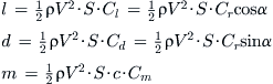
A typical presentation of change in lift coefficients with AOA is shown in Figure 8-3, with important properties labeled. The graph shows true wind tunnel test results for the NACA 4415 airfoil. A number of important observations can be made based on the figure.
Section Lift Coefficient, Cl
The two-dimensional lift coefficient is commonly called the section lift coefficient. This concept is of great importance to the airplane designer and will be discussed at length later. One of this concept’s most useful properties is that it can indicate both the effective angle-of-attack of the airfoil and how close to stalling it is.
Maximum and Minimum Lift Coefficients, Clmax and Clmin
The largest and smallest magnitudes of the lift coefficient are denoted by Clmax and Clmin, respectively. The former always has a positive magnitude and the latter a negative one. These values are extremely important because they dictate the stalling speed (at positive and negative loading) of the aircraft (and therefore wing size and airplane weight), as well as impacting other important characteristics such as the maneuvering loads and spin behavior. Generally, the stall is defined as the flow conditions that follow the first lift curve peak, which is where the Clmax (or Clmin) occurs [2, p.1].
Lift Curve Slope, Clα
Clα indicates how rapidly lift changes with angle-of-attack. The maximum value of the slope is predicted by linear thin airfoil theory for incompressible flow to be 2π (approximately 6.283) and most airfoils indeed achieve a value close to that. For instance, the slope of the red dotted line displaying the linear range in Figure 8-3 is approximately 5.90. The lift curve slope is usually linear at low AOAs; however, it is nonlinear outside this range and can have a negative slope. A nonlinear lift curve slope is indicative of flow separation prevailing on the body.
Angle-of-attack at Zero Lift, αZL
This refers to the angle-of-attack at which the airfoil produces no lift. It is important when considering wing washout (see Section 9.3.5, Wing twist – washout and washin, ϕ) and when converting the two-dimensional lift curve to three dimensions, as the change can be approximated by, effectively, rotating the lift curve around this point, toward a shallower slope (see Section 9.5.5, Step-by-step: Transforming the lift curve from 2D to 3D). The αZL is shown in Figure 8-4.

Linear Range
The linear range (here shown ranging from AOA = −12° through 8°) is called so because, within it, one can estimate the lift coefficient for any AOA using a simple linear expression, such as the one below:
![]() (8-10)
(8-10)
The extent of this region ultimately depends on the geometry and the operational airspeeds (via Reynolds numbers as discussed in Section 8.3.4, The effect of Reynolds number).
Cl at Zero AOA, Clo
Clo is the value of the lift coefficient at zero AOA. This is of great importance in the selection of the airfoil as it will affect the angle-of-incidence at which the wing must be mounted. Generally, this value ranges from 0.0 (for symmetric airfoils) to 0.6 (for highly cambered airfoils). It is negative for under-cambered airfoils (e.g. airfoils used near the root of high subsonic jet aircraft). If the AOA of zero lift, αZL, and lift curve slope, Clα, are known, the value of Clo can be calculated from:
![]() (8-11)
(8-11)
Minimum Drag Coefficient, Cdmin
Cdmin is the lowest value of the drag coefficient that can be found on the drag polar. Its magnitude is vital to the selection of the airfoil. Ideally, Cdmin should be a low as possible, but it also has to be low where it counts; in the region of intended lift coefficient of cruise.
Lift Coefficient of Minimum Drag, Clmind
Clmind is the lift coefficient where the minimum drag coefficient occurs on the drag polar. This location impacts the selection of the airfoil for the same reason as Cdmin.
8.1.5 The Pressure Coefficient
The pressure coefficient is of considerable importance in the discussion that follows, so a brief review is warranted. It is very useful to represent pressure in terms of a dimensionless quantity, similar to that of lift and drag. The incompressible pressure coefficient is defined as follows:
![]() (8-12)
(8-12)
where
q = dynamic pressure, in lbf/ft2 or N/m2
p = pressure, in lbf/ft2 or N/m2
p∞ = far-field pressure, in lbf/ft2 or N/m2
The incompressible pressure coefficient can also be written as follows:
![]() (8-13)
(8-13)
The maximum possible value of the Cp at the stagnation point in incompressible flow is 1. The Cp in compressible flow can become larger than 1 if the flow is supersonic. The compressible Cp is given by:
![]() (8-14)
(8-14)
where
Derivation of Equation (8-14)
Using the equation of state (p = ρRT), the speed of sound can be found from:
![]()
Therefore, the dynamic pressure can be written as follows:
![]()
Inserting this into Equation (8-12) yields:
![]()
QED
The Canonical Pressure Coefficient
The canonical pressure coefficient is regarded by many as a better way to represent airfoil pressure distribution. The concept was introduced by A. M. O. Smith [3] to evaluate the adverse pressure gradient and help determine the onset of flow separation. The approach scales the pressure coefficient, so it varies between 0 and 1. This is done by selecting the peak pressure (at the start of the adverse pressure gradient, i.e. where pressure begins to increase). The canonical pressure coefficient is defined as follows:
![]() (8-15)
(8-15)
8.1.6 Chordwise Pressure Distribution
The distribution of pressure along the surface of an airfoil is of fundamental importance for a number of reasons. These range from the determination of structural loads to the magnitudes of drag, lift, pitching moment, shock formation, laminar-to-turbulent boundary layer transition, hinge moments, and many other characteristics.
The pressure distribution is usually shown using the pressure coefficient (see Section 8.1.5, The pressure coefficient) plotted separately for the upper and lower surfaces (for instance, see the solid and dashed curves in Figure 8-5, respectively). For clarity, the pressure distribution for the upper surface is plotted above the one for the lower surfaces. Since the pressure coefficients are normally negative for the upper surface, the vertical axis is inverted, with the negative values above the positive ones.
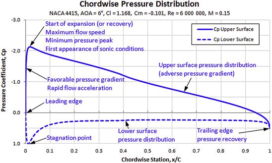
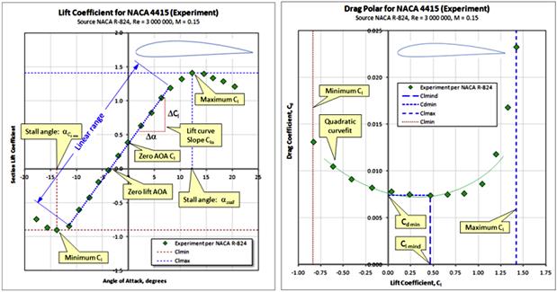
“Conventional” Lift Distribution
Figure 8-6 shows a pressure distribution generated by a conventional cambered airfoil (the NACA 4415) at a subsonic condition and an AOA of 2°. The thick solid line shows the pressure along the upper surface and the dashed one along the lower surface. It is evident that, at this AOA, the pressure on the upper surface reaches its lowest value relatively close to the leading edge, or around 20% of the chord length. This means that a favorable pressure gradient extends only as far aft as 20%. In other words, assuming a smooth surface, the laminar boundary layer is promoted only over the first 20% of the chord length. This does not mean a transition will occur immediately thereafter, but this is very likely unless the surface of the airfoil is super-smooth.

Also note that the pressure distribution along the lower surface starts with stagnation condition (Cp = 1 at x = 0), which then develops into a low-pressure dip near the 10% of the chord. This is caused by the airflow accelerating around the curved geometry in the area of the leading edge. It highlights that if curvature is present in a fluid flow, the local pressure will always be reduced – an important fact to keep in mind when trying to reduce hinge moments of control surfaces.
Figure 8-6 also shows the pressure differential (difference between the upper and lower surface pressure). It is negative along the entire chord, indicating all segments of the chord are contributing to the lift, albeit in different capacities. For instance, it is evident that the first 50% of the chord contributes substantially more to the overall lift of the airfoil than does the remaining 50%. This fact begs the question: is it possible to design an airfoil whose chordwise distribution would be uniform? Such an airfoil would have to be the most efficient possible, because all chordwise stations would contribute equally, right? Well, strictly speaking the answer is yes, although this is not achievable in reality due to the tendency of air to separate. However, airfoils that attempt this have been designed and are already in use in many aircraft, in particular, sailplanes and high-performance composite GA aircraft. A discussion of their pressure distribution follows.
Stratford Distribution
In contrast, consider the chordwise distribution of the NLF(1)-0414F airfoil shown in Figure 8-7 at the same AOA of 2°. This distribution forms a distinct flat pressure contour on the upper surface. This contour is commonly referred to as a “rooftop” or Stratford pressure distribution. Such a distribution promotes an extensive laminar boundary layer, provided the surface is sufficiently smooth.
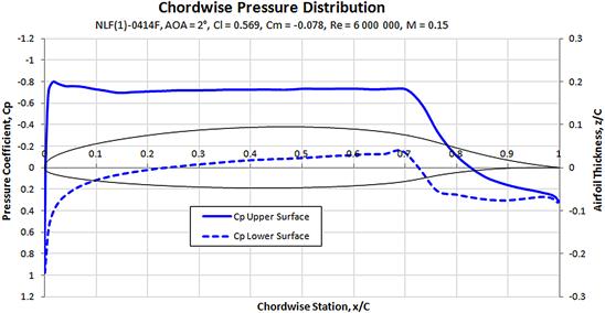
FIGURE 8-7 The chordwise distribution for an NLF airfoil at AOA = 2°. The solid line shows the Stratford distribution.
Consider a hypothetical pressure distribution that is uniform along the chord of the airfoil, from the LE to the TE. This would yield the most efficient generation of lift, as each chordwise segment is contributing equally to the total lift of the airfoil. Such a pressure distribution, on the other hand, is physically impossible because this would require the air pressure to change from a low to ambient pressure instantaneously. In real applications, the air pressure must be allowed to rise over a given distance. If the distance is too short, a separation will occur. If the distance is too long, full advantage is not taken of the benefits of the laminar boundary layer. If the distance is just right, the flow will be on the verge of separation and the flat roof will extend as far aft as possible and skin friction drag will be optimized for that airfoil. Modern airfoils are specifically designed to generate a chordwise pressure distribution along the upper surface that is uniform across much of the chord. However, this can only be achieved for a small range of specific AOAs (say 1°–2°). For this reason, it is imperative to define the mission of the aircraft clearly so the AOA at which it will be operated can be determined and used to design the airfoils.
8.1.7 Center of Pressure and Aerodynamic Center
Center of Pressure
As has already been stated, a body immersed in fluid flow induces a pressure field that, in turn, generates a resultant force and moment. The magnitude of the moment depends on the position on the body about which it is measured. Then, the center of pressure is defined as the point where the magnitude of the moment equals zero.
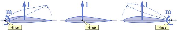
To better explain the concept, consider the three identical airfoils shown in Figure 8-8, all of which feature hinges in different places; one on the leading edge (left), the next at the center of pressure (center), and the trailing edge (right). Considering the leftmost airfoil, the lift force generates a moment that will rotate it leading edge down (counter-clockwise). By the same token, the rightmost airfoil, which is hinged at the trailing edge, would be rotated in the opposite direction: leading edge up (clockwise). It follows there must be a point between the leading and trailing edge about which no rotation would take place. This point is the center of pressure. Its location depends on the distribution of pressure along the airfoil and will change with AOA.
Aerodynamic Center and Quarter Chord Moment
The aerodynamic center is the point on a body about which the aerodynamic moment is independent of the AOA. Its presence is plotted in all standard NACA wind tunnel test graphs, where its consequence can be seen as the pitching moment curve that is constant over almost the entire α-sweep range. If the slope of the lift curve, ![]() , and the pitching moment about the quarter chord,
, and the pitching moment about the quarter chord, ![]() , are known, the aerodynamic center can be computed from:
, are known, the aerodynamic center can be computed from:
![]() (8-16)
(8-16)
The pitching moment of airfoils is often reported at the aerodynamic center, although it is needed at the quarter-chord for many stability and control problems. The following expression can be used to transfer the moment from the aerodynamic center to the quarter chord:
![]() (8-17)
(8-17)
Derivation of Equation (8-16)
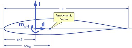
Based on Figure 8-9, the moment about the aerodynamic center can be obtained by summing the forces (l) and moments (m) as follows:
![]()
Dividing through with q·S·c, where ![]() and by referencing Equation (8-6), this can be written in a coefficient form as shown below:
and by referencing Equation (8-6), this can be written in a coefficient form as shown below:
![]()
This can easily be solved for ![]() to give Equation (8-17). Then, differentiating with respect to α and recalling that the definition of the aerodynamic center means that the change in moment with change in α is zero, this above is rewritten as shown:
to give Equation (8-17). Then, differentiating with respect to α and recalling that the definition of the aerodynamic center means that the change in moment with change in α is zero, this above is rewritten as shown:
![]()
Using convention in writing the slopes and solving for xac results in the following:
![]()
QED
8.1.8 The Generation of Lift
Generally, the generation of lift can be explained in at least three ways. These are known by their casual names momentum theorem, Bernoulli theorem, and the circulation theorem. We will briefly introduce each in order to provide clarity as each is occasionally referred to in other places in the text. As an interesting side note, some people outside industry and academia have engaged in debates about the importance of the first two methods. There are some who claim that Bernoulli’s theorem is wrong and the momentum theorem is the definitive explanation, whilst others claim the opposite. While it can be argued that the momentum theory is easier for laypeople to relate to (see below), such debates are silly and only reveal the participant’s limited understanding of aerodynamics. The fact is that all three are excellent ways to describe the generation of lift and all have their pros and cons.
Momentum Theorem
The momentum theorem explains lift as the consequence of a wing moving through a mass of air and giving it a downward motion (see Figure 8-10). Since the mass of air is initially at rest, the downward motion means the vertical speed of the air changes from zero to some finite value in a given amount of time. This, in turn, means that a force will be generated in the opposite direction in accordance with Newton’s third law of motion. The magnitude of this force can be estimated using Newton’s second law of motion. The second law of motion states it is the rate of change of momentum of the mass of air that generates the force. The third law states an equal force that acts in the opposite direction of the motion of the mass is also generated. It is this force that we call lift. A common analogy used to describe this phenomenon is the recoil of a firearm. As is well known, the change in the momentum of a bullet generates a force that acts in the opposite direction of its motion. Thus, the sudden down flow imparted on the air effectively generates “continuous recoil” – the lift.
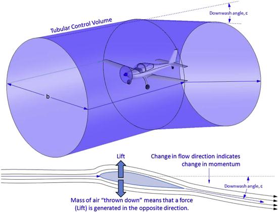
FIGURE 8-10 An airplane’s motion causes a downward deflection of a tube of air; in turn, in accordance with Newton’s second law of motion, its rate of change of momentum generates a force (lift) in the opposite direction.
The downward motion of the air is called downwash, here denoted by the letter w, and it represents the vertical speed of air behind the wing. It contrasts with the horizontal speed; a result of the wing moving through air. If we know the downwash and the mass flow of air being deflected, the magnitude of the lift can be estimated, as stated earlier, using Newton’s second law of motion:
![]() (8-18)
(8-18)
where ![]() = mass flow rate inside the cylinder = ρV·πb2/4.
= mass flow rate inside the cylinder = ρV·πb2/4.
The mass flow rate in the stream tube is given by ![]() , where Atube is the cross-sectional area of the stream tube. If it is assumed that the diameter of the stream tube in Figure 8-10 equals that of the wingspan (denoted by b) then the rate of change of momentum (lift force) can be estimated from:
, where Atube is the cross-sectional area of the stream tube. If it is assumed that the diameter of the stream tube in Figure 8-10 equals that of the wingspan (denoted by b) then the rate of change of momentum (lift force) can be estimated from:
![]() (8-19)
(8-19)
Equating this with the standard expression for lift (Equation (8-6)) allows the magnitude of the downwash to be estimated:
![]() (8-20)
(8-20)
Noting that S = b·Cavg and AR = b/Cavg this can be rewritten as follows:
![]() (8-21)
(8-21)
Since the downwash can approximated by w = εV (see Figure 8-10), we can write:
![]() (8-22)
(8-22)
This equation leads to another result, which as will be shown later, is very helpful in stability and control theory:
![]() (8-23)
(8-23)
Bernoulli Theorem
The Bernoulli theorem has been used for decades to explain the formation of lift to generations of engineers and pilots. It postulates that lift is the consequence of the difference in pressure between the upper and lower surfaces of an airfoil, although this would more properly be explained as the resultant of integrating the pressure over the entire surface of a body. Named after the Swiss mathematician Daniel Bernoulli (1700–1782), the theorem stipulates there is a relationship between the pressure and speed of the fluid at a point and along a streamline that goes through that point. This is expressed as follows:
where
g = acceleration due to gravity, in ft/s2 or m/s2
p = pressure, in lbf/ft2 or N/m2
z = elevation above or below some reference plane, in ft or m
ρ = fluid density, in slugs/ft3 or kg/m3
γ = ratio of specific heat for the fluid (1.4 for air at altitudes below 100 km).
Bernoulli’s theorem is used daily by thousands of people in industry and academia to estimate the aerodynamic forces acting on a body. Computational fluid dynamics (CFD) software uses the theorem to estimate aerodynamic forces and moments acting on a body with great success.
Kutta-Joukowski Circulation Theorem
The Kutta-Joukowski circulation theorem is much more a mathematical method than it is an explanation. Named after the German mathematician Martin Wilhelm Kutta (1867–1944) and the Russian scientist Nikolay Yegorovich Joukowski1 (1847–1921), the theorem postulates that the lift generated by an airfoil can be considered the product of density (ρ), forward airspeed (V), and a mathematical concept called circulation (Γ). In short, the Kutta-Joukowski theorem states that the airfoil’s lift can be expressed as follows:
![]() (8-26)
(8-26)
where the circulation is calculated using the expression [4]:
![]() (8-27)
(8-27)
where
![]() = velocity (see Figure 8-11)
= velocity (see Figure 8-11)
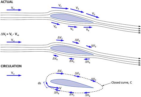
FIGURE 8-11 The top image shows the actual airflow over a wing and that the airspeed along the upper surface the wing is faster than along the lower surface. Assuming the speed at each point is known, the total value can be subtracted from the far-field velocity. This is shown in the center image and reveals that there is a general flow backwards along the upper surface and forward along the lower. This motion is reminiscent of a circulation around the airfoil, shown in the bottom image.
C = closed curve in a flow field (see Figure 8-11)
To better understand the concept of circulation, consider Figure 8-11, which shows the airflow around an airfoil. The top figure shows the far-field airspeed, V∞, and some representative airspeed V1 through V6, positioned at selected locations in the flow-field, above and below the airfoil. Then, it is possible to calculate the difference between each of those airspeeds and the far-field airspeed. This is shown as the airspeeds ΔV1 through ΔV6 in the center figure. The important observation is that the airspeed differences along the upper surface are positive and point in the flow direction. Conversely, they are negative along the lower surface and point in a direction opposite that of the general airflow. As can be seen in the bottom figure, these differentials effectively form a path around the airfoil. This path is the circulation.
The Kutta-Joukowski theorem is very useful in a number of computational fluid dynamics (CFD) methods, such as the lifting line method (see Section 9.7.1, Prandtl's lifting line theory), and the vortex-lattice methods, where it is directly used to estimate the lift and induced drag force generated by a lifting surface.
8.1.9 Boundary Layer and Flow Separation
An understanding of the nature of fluid as it moves over a surface is imperative in aircraft design. This is not only true to explain a number of phenomena that occur on airplanes in flight, but also when wind tunnel testing a scaled model of a larger aircraft and interpreting the results. Much of this understanding is borrowed from boundary layer theory (BLT), which describes the nature of viscous flow near the surface of a body through expressions developed using conservation laws and the Navier-Stokes equations. This theory is extensive and while essential to treatment of viscous fluid flow, it is too large in scope to be suitable for this book. For this reason, for theoretical derivations refer to texts such as those of Schlichting [5] and Young [6]. Only important results will be presented in this text.
Reynolds Number
The Reynolds number (Re) is a measure of the ratio of inertial forces to viscous forces in a fluid flow. It is of great importance in the analysis of the boundary layer. It is defined as follows:
![]() (8-28)
(8-28)
where
L = reference length (e.g. wing chord being analyzed), in ft or m
V = reference airspeed, in ft/s or m/s
A simple expression, valid for the UK system at sea-level conditions only, is (V and L are in ft/s and ft, respectively):
![]() (8-29)
(8-29)
For the SI system at sea-level conditions only, the expression becomes (V and L are in m/s and m, respectively):
![]() (8-30)
(8-30)
The Effect of Flow Separation
Consider two identical aircraft whose only difference is size or scale. Imagine these are immersed in fluid flow at an identical airspeed such that, as far as the aircraft is concerned, it differs in Reynolds numbers only. Now consider them rotated slowly through an alpha-sweep, from 0° to 90°, while we collect their force and moment coefficients. At first, while the flow is mostly attached, both aircraft will effectively generate identical and linear force and moment coefficients. However, after some AOA (perhaps at α = 8°) has been reached, the flow begins to separate on the smaller body, while it remains attached on the larger one. The resulting force and moment coefficients for the small body now turn nonlinear, while remaining linear for the larger one. Eventually, the larger body too begins to experience the same effect (perhaps at α = 12°). The flow separation causes a large increase in drag and reduction in lift. The pitching moment may increase or reduce depending on the overall geometry. This calls for a distinction in the nature of the flow over the two bodies. Generally, three such types are identified, based on the character of the boundary layer that envelopes the body. They are called laminar, turbulent, and separated flow (see Figure 8-12).
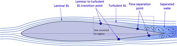
FIGURE 8-12 Three types of fluid flow: laminar, turbulent, and separated on an airfoil. See Figure 8-13 for the zoomed-in region.
Boundary Layer Transition
A body moving in a fluid will generally be exposed to three distinct types of fluid flow; one is characterized by the presence of a laminar boundary layer, another by a turbulent boundary layer, and the third by separated flow which contains molecules that flow in all possible directions, even upstream (see Figure 8-13). A laminar boundary layer occurs when the streamlines inside the boundary layer flow smoothly. In contrast, streamlines inside a turbulent boundary layer are chaotic. An important phenomenon takes place as the initially laminar boundary layer changes to a turbulent boundary layer, due to a process called transition. When the airflow strikes a smooth body a laminar boundary layer will form immediately, but will later degenerate when it transitions into a turbulent boundary layer. This generally occurs when the local Reynolds number equals approximately 5 × 10⁵. This is referred to as the transition Reynolds number.
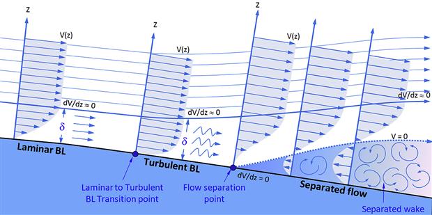
FIGURE 8-13 The nature of fluid flow inside laminar and turbulent boundary layers, and separated flow.
Unfortunately, the transition is complicated by factors that may change the transition Reynolds number and may cause the transition to happen at a different (lower or higher) Reynolds number [7]. Note that the term early transition means that the transition takes place earlier than indicated by the value of the Reynolds number. By the same token, delayed transition refers to the opposite. Factors that may change the Reynolds numbers:
(1) Surface roughness. The transition process is dependent on flow disturbances that take place inside the boundary layer. For this reason, the presence of small surface imperfections (roughness) will excite these disturbances and expedite the transition – even to very low values of the Reynolds number. Also see Section 8.3.13, The effect of leading edge roughness and surface smoothness.
(2) Surface temperature. The thickness of the boundary layer increases with temperature, as does the energy contained within it. The increase in temperature and thickness is associated with an earlier transition. A cold surface tends to delay transition.
(3) Pressure gradient. A favorable pressure gradient (i.e. a reduction in static pressure along the flow direction, which is caused by flow acceleration) will stabilize the laminar boundary layer and delay transition. The opposite holds for an adverse pressure gradient (i.e. an increase in static pressure associated with a flow deceleration). Also see Section 8.1.6, Chordwise pressure distribution and Figure 15-14.
(4) Mach number. The transition Reynolds number increases with higher Mach number (i.e. in compressible flow).
Flow Separation
In a separated flow the streamlines are separated from the surface. Such flow may actually flow upstream, against the direction of the free stream airflow. Flow separates when the gradient dV/dz equals zero on the surface (z = 0). The external geometry of an airplane should be shaped so the areas of flow separation at the mission condition are minimized, if not eliminated.
All three types usually manifest themselves in fluid flow in the order shown in Figure 8-13. This typically occurs on bodies as shown in Figure 8-14 or Figure 8-15. The former shows flow over an object that features a rounded, small-radius leading edge (LE). The flow forms a laminar boundary layer on the forward part of the object (the bow), followed by a transition to a turbulent boundary layer, and, finally, by the flow separating into a turbulent wake at the stern. Note that the streamlines outside the boundary layer are smooth and can be treated as if they belonged to an inviscid fluid. In fact, for computational efficiency, this is how most Navier-Stokes solvers treat fluid flow: viscid inside the boundary layer, but inviscid outside of it.
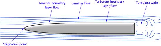

FIGURE 8-15 Flow over a blunt LE object results in an immediate forward flow separation, subsequent reattachment, and finally, a turbulent wake. The forward flow separation region is called a “separation bubble.”
Figure 8-15 shows a different scenario, in which an object with a very blunt LE causes flow separation on the LE that results in (highly) turbulent, circulatory flow inside the flow separation region. The laminar streamlines flowing over this region attach aft of this region before separating into the turbulent wake at the stern.
The forward flow separation region is usually referred to as a “separation bubble.” Such bubbles can also form on objects that are considerably less blunt than the one in Figure 8-15. They can even occur on airfoils if their geometry is conducive to such formation. This may be caused by sudden change in curvature. Besides an increase in drag, separation bubbles on airfoils may lead to very detrimental stall characteristics.
Separation bubbles can occur on any aircraft, in particular at the wing/fuselage juncture. However, the phenomenon also occurs on lifting surfaces, in particular on small chords (or low Reynolds numbers). As discussed in Section 8.2.10, Famous airfoils, The NACA 23012 airfoil is used for a number of GA aircraft in spite of its abrupt stall characteristics, which are attributed to the formation of a separation bubble. But they are a prevalent problem for even smaller Reynolds numbers, such as those in which radio-controlled aircraft operate (60,000–500,000). In this region a stable bubble may form in the laminar boundary layer along the leading edge of the wing, increasing the drag of the vehicle. This is referred to by many as “bubble drag” [8]. One way of reducing this drag is to design the airfoil such that its transition ramp2 reduces the chance of a bubble formation (refer to Ref. [8] for more details). Another way is to place a transition strip (often called a “trip strip”) along the leading edge to force the laminar boundary layer to transition into a turbulent one without forming the separation bubble. Currently this is a trial-and-error approach and a trip strip that is ideal for one Reynolds number may be detrimental for another one. Research shows their effect is contingent upon the size of the bubble, its intensity, AOA, and geometry of the airfoil.
Factors Affecting Laminar Flow
The laminar boundary layer is very sensitive to a number of factors. Some are out of the control of the designer, whereas others are not and, effectively, depend on his awareness. Among those are (list partially based on Bertin [9]):
1. Geometry (e.g. sweep and surface curvature).
2. Surface smoothness (or lack thereof).
4. Compressibility effects (Mach number, Reynolds number).
5. Atmospheric conditions (ice crystals, rain).
6. Manufacturing quality (waviness, smoothness, steps and gaps in surface joints).
7. Leading edge quality (insects, dirt, erosion, icing).
8. Suction or blowing at the surface (surface openings, distribution of boundary layer control).
8.1.10 Estimation of Boundary Layer Thickness
The estimation of the thickness of the boundary layer has many applications. As an example, it is essential in the design of boundary layer diverters for jet engine installation. It is also used in many computational fluid dynamics applications, when fluid flow is being modeled as inviscid and the geometry of the immersed body must be modified (enlarged) to account for the thickness of the viscous layer.
The thickness of the boundary layer depends on whether it is laminar or turbulent. A turbulent boundary layer grows at a faster rate and is thicker than a laminar boundary layer at the same conditions. Their thicknesses can be estimated from (based on Ref. [9]):

8.1.11 Airfoil Stall Characteristics
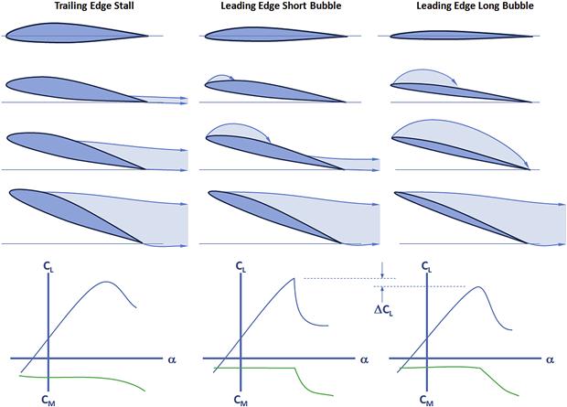
In this text, stall refers to the flow condition that follows the first peak of the lift curve. It is a consequence of the formation of a large separation located between the leading and trailing edges of the airfoil. The thickness of the airfoil largely dictates how flow separation develops on the airfoil. If the airfoil is thick, the separation tends to begin at the trailing edge and move forward as the AOA increases. On the other hand, if the airfoil is thin, the separation tends to begin at the leading edge in the form of a separation bubble. This has a profound effect on the maximum subsonic section lift coefficient as well as drag. However, other parameters besides airfoil thickness affect the maximum lift as well. Among those are the location of the airfoil’s maximum thickness, camber and its chordwise location, Mach number, Reynolds number, free-stream turbulence, and the surface condition (roughness) [2]. All affect the nature of the flow separation that ultimately places an upper limit on the maximum lift. Reference 10 classifies the nature of the flow separation in terms of trailing edge and leading edge stalls, as described below.
Trailing Edge (TE) Stall
This is undoubtedly the best known among the three types of stalls and typically occurs on thick airfoils, whose thickness-to-chord ratio is around 12% or greater [10]. Such airfoils are characterized by a smooth change in Cl and Cm between the negative and positive lift peaks (see Clmax and Clmin in Figure 8-3 and Section 8.1.4, Properties of typical airfoils) and often well beyond those. The shape of the peak of the lift curve is rounded with a mild drop in Cl. Growth in post-stall drag polar is gradual, and the pitching moment curve is without sharp breaks. The flow stays mostly attached to an AOA of about 10°, beyond which it progressively moves forward. At maximum lift the flow is separated to approximately mid-chord the rear half of the airfoil.
Leading Edge (LE) Stall
Leading edge stalls are much less familiar to the General Aviation community than TE stalls. They are associated with sharp leading edge radii of thin airfoils (which are almost never used for GA aircraft – excluding the NACA 23012 airfoil, which is used on a number of GA aircraft). The sharp LE results in a larger pressure peak than airfoils with larger radius LE. This is evident in Figure 8-17, which shows the thinner NACA 4408 airfoil peaks at Cp ≈ −16.5 versus Cp ≈ −6.0 for the thicker NACA 4415 airfoil. As a consequence, the pressure recovery, behind the peak for the thinner airfoil, is much steeper than for the thicker one. This is a problem nature solves by separating the laminar boundary layer. This separation can occur well below the AOA where the airfoil actually stalls. It forces the laminar boundary layer to transition into a turbulent one, forming a bubble of trapped low-energy air between the surface of the airfoil and the boundary layer. An example of such a bubble is shown in Figure 8-18. On a wing the bubble is a spanwise vortex.
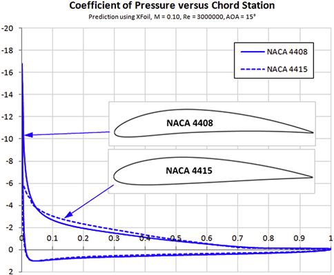
FIGURE 8-17 Chordwise pressure distribution for a thin (NACA 4408) and a thick (NACA 4415) airfoil at AOA = 15°, showing the thinner airfoil results in a much greater pressure peak than the thicker one.
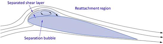
FIGURE 8-18 Formation of a separation bubble on a thin airfoil. (based on Ref. [11])
Research has shown that the bubbles come in two distinct forms, short or long, and each predicates different scenarios [11]. The difference between the two is determined using Owen’s criterion, which computes the Reynolds number of the displacement thickness of the boundary layer using the following expression:
![]() (8-33)
(8-33)
where V is the velocity at the edge of the boundary layer, ν is the kinematic viscosity and δ1 is the displacement thickness. In Ref. [12] this value was always found to be greater than 500 for a short bubble and less than 500 for a long one. Note that the size of the bubble, in effect, depends on the free stream Reynolds number, so it is possible the stall behavior of the airfoil changes from one to the other. If the Reynolds number is high enough, chances are no bubble will form. The difference between the two is as follows:
(1) Short-bubble leading edge stall: the length of the bubble is about 1% of the chord at low AOAs, but reduces in size with increased AOA. The bubble has limited effect on the pressure distribution and high peak suction can continue to rise despite the bubble’s presence up until some specific AOA, when the flow abruptly and finally separates from the airfoil’s surface. This results in a violent stall, accompanied by large change in lift and pitching moment [10].
(2) Long-bubble leading edge stall: the length of the bubble is about 2–3% of the chord at a low AOA. However, this grows rapidly with AOA until a reattachment fails to take place, causing the bubble to combine with the full flow separation over the airfoil. A long bubble will affect the pressure distribution over the airfoil in profound ways and will cause the peak suction to collapse. The maximum lift for the long bubble is less than that for the short one, but the stall is less abrupt [10].
The maximum lift coefficient of thin airfoils that stall because of flow separation at the leading edge can be determined based on the leading edge geometry. A so-called leading-edge parameter, which is defined as the difference between the upper-surface ordinates of the airfoil at the 0.15% and 6% chord stations, has been used for this purpose with good results [13] (for instance see Section 9.5.12, Step-by-step: CLmax estimation per USAF DATCOM method 2). Additional correction is required for thicker airfoils. Compressibility effects are important on thick airfoils as they cause reduction in the maximum lift coefficient starting at M ≈ 0.2. Reference [13] also presents a method to estimate the maximum lift coefficient of several airfoils. The three types of airfoil stalls are illustrated in Figure 8-19.
8.1.12 Analysis of Ice-accretion on Airfoils
Flight into inclement weather is commonplace nowadays, with aircraft being certified to fly into known icing conditions that arguably represent the greatest challenge any aircraft can be exposed to. While the engineering of ice removal is beyond the scope of this section, it is helpful for the aircraft designer to understand the fundamentals of ice-accretion on airfoils.
NASA’s Glenn Research Center has been a pioneer in the development of computational methods that estimate the collection of ice (or ice accretion) on an airfoil’s leading edge. This development included the implementation of these methods in a computer code called LEWICE (after the research center’s former name Lewis Research Center). The code accurately predicts the growth of ice under a range of meteorological conditions and, because it has been so extensively validated by NASA, is considered very reliable in industry.
Generally, such codes work as follows. First, a table containing the geometric description of the airfoil (i.e. its x- and y-coordinates) is read and analyzed using a panel-code solver. This will allow the code to determine the flow field around the airfoil, including the stagnation points. Then, the accumulation of ice at the stagnation points over a specific time (which the user may specify directly or have the program determine) is estimated. Clearly this will modify (or grow) the initial geometry and this is used to define a new geometry (i.e. the airfoil with the small amount of ice growth or accretion), which is then fed again into the solver as the input “airfoil” for the next iteration. The process is then repeated for a specified time. The user will have to specify various properties of the air during the flight condition, such as its relative humidity, liquid-water content, droplet size, temperature, airspeed, and other parameters. Figure 8-20 shows an example output from LEWICE for a common GA airfoil, the NACA 64-215. It shows that ice accretion is a formidable foe for aircraft wings.
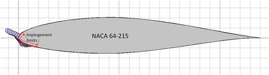
FIGURE 8-20 A LEWICE prediction showing ice accretion on an unprotected NACA 64-215 airfoil after 45 minutes exposure to supercooled liquid water at −4.75 °C (23.4 °F) at an airspeed of 90 m/s (295 ft/s) and AOA of 4°. The chord is 1.0 m (about 40 inches).
The purpose of such research is to provide aircraft manufacturers with a reliable tool to estimate what is called the impingement limits, which are points on the upper and lower surfaces beyond which limited ice accretion takes place. It must be defined to determine how far aft of the leading edge ice protection must wrap. Impingement limits are determined for a variety of flight conditions and atmospheric conditions and are ultimately based on the collectively aft-most limits.
8.1.13 Designations of Common Airfoils
A large number of different airfoils have been designed since the dawn of flight. These offer a range of properties, some ideal, while others are less desirable. As a consequence, the sheer number sometimes makes the airfoil selection process a bit daunting. The literature3 presents a number of airfoil designations that appear perplexing at first, although eventually one discovers the same airfoil designations appear repeatedly. Table 8-1 lists designations of airfoils that are found in use on various airplanes.
TABLE 8-1
Designations of Common Airfoils
| AG | Ashok Gopalarathnam, an independent airfoil designer |
| ARA | The Aircraft Research Association Ltd, Britain |
| Clark | Col. Virginius Clark of the NACA |
| Davis | David Davis, an independent airfoil designer |
| DESA | Douglas El Segundo Airfoil |
| DLBA | Douglas Long Beach Airfoil |
| Do | Dornier |
| DSMA | Douglas Santa Monica Airfoil |
| DFVLR | The German Research and Development Establishment for Air and Space Travel |
| DLR | The German Aerospace Center |
| Drela | Dr. Mark Drela of MIT |
| EC | The National Physical Laboratories, Britain |
| Eiffel | Gustave Eiffel, an early French aeronautical researcher |
| Eppler | Dr. Richard Eppler of the University of Stuttgart |
| FX | Dr. F.X. Wortmann of the University of Stuttgart |
| GU | University of Glasgow in Scotland |
| Gilchrist | Ian Gilchrist of Analytical Methods Inc. |
| Gottingen | The AV Gottingen aerodynamics research center in Germany |
| Joukowsky | Nicolay Egorovich Joukowsky, an early Russian aeronautical researcher |
| K | Dr. Yasuzu Naito of Nakajima |
| LB | Dr. Ichiro Tani of Tokyo University |
| Liebeck | Dr. Robert Liebeck of McDonnell Douglas, now Boeing |
| Lissaman | Dr. Peter Lissaman of AeroVironment Inc. |
| MAC | Airfoils designed at Mitsubishi. During the 1940s, the designer was Tsutomu Fujino |
| McWilliams | Rick McWilliams, an independent airfoil designer |
| Narramore | Jim Narramore of Bell Helicopter Textron |
| NACA | The US National Advisory Committee for Aeronautics |
| NASA | The US National Aeronautics and Space Administration |
| NN | Dr. Hideki Itokawa of Nakajima |
| NPL | The National Physical Laboratories, Britain |
| Navy | The US Navy, Philadelphia Navy Yard |
| Onera | The French National Aerospace Research Establishment |
| RAE | The Royal Aeronautical Establishment, Britain |
| RAF | The National Physical Laboratories, Britain |
| Riblett | Harry Riblett, an independent airfoil designer |
| Roncz | John Roncz, an independent airfoil designer |
| Selig | Dr. Michael Selig of the University of Illinois, Urbana-Champaign |
| Somers | Dan Somers of Airfoils Inc. |
| TH | Dr. Tatsuo Hasegawa of Tachikawa |
| TsAGI | The Russian Central Aerodynamics and Hydrodynamics Institute |
| USA | The US Army |
| Viken | Jeff Viken of NASA Langley Research Center |
Primarily based on http://www.public.iastate.edu/∼akmitra/aero361/design_web/airfoil_usage.htm.
8.1.14 Airfoil Design
During the history of aviation, thousands of different airfoils have been designed for applications ranging from aircraft, turbo machinery, wind turbines, propellers, and even ships (hydrofoils). It is likely that a useful airfoil for a new design may be found in that database. However, the modern manufacturer of aircraft will instead often opt for airfoils specifically designed for new aircraft. This way, the new airfoil may have a higher maximum lift than the older airfoil, but this also guarantees the aircraft can truly operate at a minimum drag during its cruise mission. The latter can have a profound impact on the bottom line for the customer and result in substantial savings in fuel costs in the process, making the airplane more marketable. The cost of designing an airfoil is usually a minor expenditure of the complete development program, in particular for commercial aircraft, and is therefore something that should be seriously considered at the beginning of the design process.
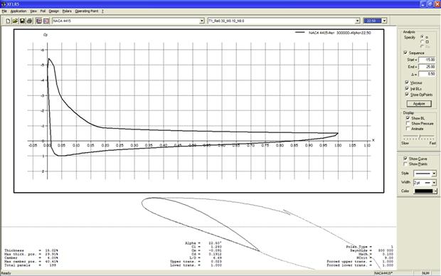
Airfoils are typically designed by two means; direct analysis and inverse design. Nowadays, this is always done using computer software. Two-dimensional computer programs such as Xfoil [14]; XFLR5 (this program is actually a user-friendly interface for Xfoil, which it runs in the backround) [15]; the Eppler Code [16]; or AeroFoil [17], are widely used and run on any personal computer (PC). Two of these, Xfoil and XFLR5, are even distributed free of charge. All of the following programs allow polars (CL versus α, CD versus CL, etc.) to be plotted and airfoils to be designed using an inverse design method.
Xfoil and XFLR5
Xfoil is probably the best known of the above codes. It dates back to 1986 and was written by Dr. Mark Drela, an aerodynamics professor at the Massachusetts Institute of Technology. It uses a high-order panel method and a fully-coupled viscous/inviscid interaction method to evaluate drag, boundary layer transition and separation. Xfoil is widely used in the aircraft industry and generally speaking is a reliable tool, although, in the view of this author, it suffers from a poor user interface when compared to many other codes. The user of modern computer operating systems is averse to the unfriendly interfaces of the bygone MS-DOS era. This has been solved in a program called XFLR5 [18], developed by Mr. André Deperrois, which makes Xfoil analyses much easier to perform (see Figure 8-21).
Xfoil allows the user to perform viscous and inviscid analysis of existing airfoils. The user can specify where a laminar boundary layer transitions into a turbulent one, or have the program predict the movement of the transition point with AOA. The viscous analysis can be used to predict Cl, Cd, and Cm to just beyond Clmax, and uses Karman-Tsien compressibility correction at high subsonic airspeeds (see Section 8.3.6). The program allows the user to simulate control surface deflection by specifying hinge point and deflection angle.
PROFILE (“The Eppler Code”)
The software PROFILE was written by Dr. Richard Eppler of the University of Stuttgart and Dan Somers, a consulting aerodynamicist. The program uses a conformal-mapping method for the design of airfoils for low-speed applications with prescribed velocity-distribution characteristics. The program is claimed to be user-friendly by the distributer of the program, www.airfoils.com/.
AeroFoil
The software AeroFoil was developed by Mr. Donald Reid, a professional nuclear engineer who has a background in aerospace engineering, and “is intended to be the most ‘user-friendly’ of its type,” as stated on its website, aerofoilengineering.com/index.htm. The software uses a vortex-panel method coupled with integral boundary layer equations to calculate the aerodynamic properties of airfoils. It allows up to three airfoils to be compared simultaneously. Validation examples are provided on the website and show the predictions made by the program are in good agreement with experiment.
JavaFoil
JavaFoil is simple and easy-to-use software developed by the German aerodynamicist Dr. Martin Hepperle. The program performs a potential flow analysis using a higher-order panel method, in which the vorticity varies linearly along each panel representing the airfoil. Then, an integral boundary layer method is applied, using a separate boundary layer analysis module. Beginning at the stagnation point, the method solves a set of differential equations to help evaluate the characteristics of the boundary layer. According to information on the developer’s website, the equations and criteria for transition and separation were developed by Dr. Eppler. The program is free and available from www.mh-aerotools.de/airfoils/javafoil.htm. It provides a routine that allows a large number of airfoils to be generated.
Design Process
Once a decision has been made to design an airfoil, the first step in the design is to list the desired characteristics. Such a list can consist of a range of operational lift coefficients and conditions (Mach number, Reynolds number) at which specific properties such as maximum value of the lift should occur, desirable entry into the post-stall region, or where minimum drag should occur, extent of laminar flow, the magnitude of the pitching moment coefficient, as well as desirable geometric characteristics such as thickness and its location along the chord. The next step is to decide on a methodology: direct or inverse method (see below). Some designers use existing airfoils as a baseline and modify them, typically using both methods and a trial-and-error approach until most of the desired characteristics have been achieved.
Direct Analysis Method
A direct analysis is the evaluation of the pressure field around an airfoil that has already been defined. In direct analysis the ordinates of the airfoil are entered into software such as Xfoil, PROFILE, or AeroFoil and then the software will predict lift, drag, and pitching moment of the airfoil at the angles-of-attack specified. The most important feature of such software is an accurate prediction of flow separation growth with AOA, subsequent stall, and width and depth of the drag bucket at lower AOA. The software packages cited above are all capable of such predictions, although the accuracy of the results is not being commented on. The software cited sometimes yields different predictions for an identical airfoil at identical conditions. It is always the responsibility of the user to learn to properly use the software and this requires the predicted results to be compared with reliable wind tunnel tests.
The direct analysis method is not an ideal way to design an airfoil for a desired pressure distribution, as this would require substantial trial and error to accomplish. The inverse airfoil design method discussed below is a far better approach.
Inverse Airfoil Design Method
The inverse method allows the airfoil designer to specify a specific velocity distribution along the surface, which is then used to calculate the geometry that will generate such a distribution. The knowledgeable designer will know the consequences of a specific speed distribution, where it will promote laminar flow or cause early separation, and so on. For this reason, airfoil design is a field of specialization and calls for the evaluation of large numbers of airfoils to build a database of behavior based on experience. Inverse methods were responsible for significant advances in airfoil design in the 1950s, when enough computational power was realized to allow integral boundary layer methods to be coupled with potential-flow solutions. The computational prowess of the modern computer is now used to implement such methods using the full Navier-Stokes equations.
8.2 The Geometry of the Airfoil
This section presents important properties of the geometry of the airfoil and a number of famous airfoils the aircraft designer should be aware of, as some offer interesting possibilities, while others should be avoided.
8.2.1 Airfoil Terminology
The discussion of airfoils in this text assumes the designer is familiar with the concepts defined below in Figure 8-22 and Figure 8-23.


Thickness, Mean-line and Camber
NACA defines airfoils based on a specific thickness distribution and mean-line. The camber is defined as the maximum distance between the mean-line and the chordline. Camber strongly affects the downwash behind the airfoil and, thus, how much lift is generated. The rule-of-thumb is that the larger the camber, the greater the maximum lift of the airfoil and greater the thickness the greater the stall angle-of-attack and drag. Of course there are exceptions. Generally, the greater the camber the greater is the drag as well.
LE Radius
The leading edge radius impacts the maximum lift of the airfoil, as well as its drag in cruise. Generally, the larger the radius the more lift will be generated at high AOA, as this delays flow separation near the LE. This often manifests itself as a less abrupt reduction in lift at stall (“stall break”). Large radius can also increase the airfoil’s drag, although this is also dependent on the geometry of the airfoil downstream.
Square TE
A square trailing edge is sometimes employed to decrease adverse pressure gradients4 on airfoils. This is important for NLF airfoils (which feature the maximum camber way back along the chord) to help stabilize the boundary layer on the aft part of the airfoil. This way, the formation of a separation bubble is prevented and, consequently, both lift and drag characteristics are improved. It is of importance how the TE is squared. A sharp trailing edge cannot just be made blunt, as this will not increase the thickness of the airfoil upstream. Rather, the TE must be deliberately thickened to improve adverse pressure gradients. Blunt TE airfoils are sometimes called “flatbacks.”
Geometric Description
The geometric description of airfoils is generally given in so-called ordinate tables. Such tables often list the airfoils upper and lower surfaces separately in terms of x and z coordinates. The x-axis is called the chord line and the x-ordinate represents the chordwise station and the z-ordinate the height above or below the x-axis. Then we define the mean-line and thickness as follows:
![]() (8-34)
(8-34)
![]() (8-35)
(8-35)
If the mean-line and thickness are tabulated rather than the ordinates, then these can be obtained from:
![]() (8-36)
(8-36)
![]() (8-37)
(8-37)
8.2.2 NACA Four-digit Airfoils
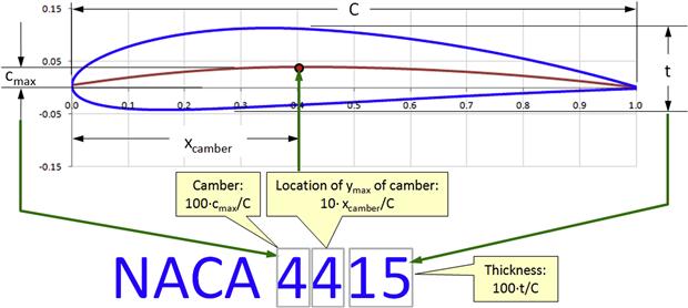
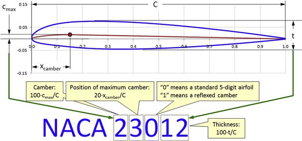
The NACA four-digit airfoils were the product of Eastman N. Jacobs and his colleagues at the NACA Variable-Density Wind Tunnel, who around 1929 demonstrated that the characteristics of an airfoil are largely dependent on its thickness and mean-line [19]. This allowed the airfoils to be described using a mathematical formulation and a designation system that reflects the airfoil’s geometric properties. These airfoils have designations like 2412, 3308, or 4415 (see Figure 8-24). The figure shows how the digits are interpreted. Further development of these airfoils for propellers was done by Albert von Doenhoff [20]. The development NACA 4-digit series airfoils are detailed in Refs [19,20].
Applications
The airfoils are widely used in GA aircraft, with the best-known aircraft being a family of Cessna airplanes. Cambered versions are used for wings, while symmetric ones are used for HT and VT. Symmetric airfoils are also used for helicopter rotors, antennas, and even for some supersonic aircraft and missile fins.
Numbering System
As shown in Figure 8-24, the numbering system is based on the geometry of the airfoil. The first digit indicates the camber in percentage of chord. The second digit indicates the distance from the leading edge to the maximum value of the camber in tenths of the chord. The last two digits indicate the thickness of the airfoil in percent of the chord. Thus, the NACA 4415 airfoil has a 4% camber located at 40% of the chord and is 15% thick. Also, NACA 0009 is a symmetrical airfoil as indicated by the first two digits 00. The airfoil is 9% thick.
Computation of Airfoil Ordinates
The geometry of the airfoil can be determined by computing the x- and y-values in accordance with the Step-by-step that follows. The algorithm is based on the report NACA TN-460 and is set up for analysis using a spreadsheet. Note how the ordinates of the upper and lower surfaces are calculated. These are rotated with respect to the slope of the mean-line. Thus, the x-value of the point on the upper surface is not the same as that of the point on the lower surface. This necessitates the evaluation of the slope of the mean-line and the rotation about the point (x, yc) as shown in Figure 8-25.
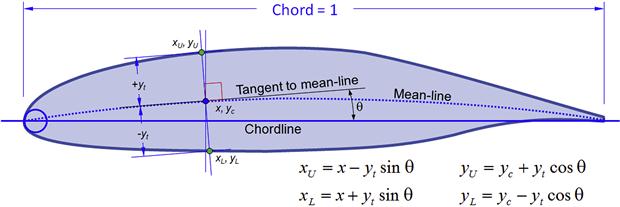
FIGURE 8-25 Determination of the ordinates for the upper and lower surfaces of a NACA 4-series airfoil.
The definition of airfoil is always based on the assumption that the leading edge is located at x = 0 and the trailing edge at x = 1. The resulting chord is of a unit length. The advantage of defining the airfoil in terms of a unit chord is that it can be easily scaled up by a direct multiplication of the ordinates by the desired chord. The geometric definition is in the form of a table containing the x- and y-coordinates of the airfoil. As stated in the previous section, such a table is called an ordinate table, where the word ordinate refers to the y-value of a specific co-ordinate.
The ordinate table lists the x-values for the airfoil by distributing them along the x-axis. While the x-values are sometimes distributed uniformly, a more desirable distribution is based on a cosine scheme as shown in Figure 8-26. Doing so will guarantee a better definition of the leading edge, where curvature is greater. This scheme consists of a unit circle, which is uniformly sectored at an angle Δϕ. The value of Δϕ is determined from the number of points as follows:
![]() (8-38)
(8-38)
Now consider the thick dark line extending from x = −1 to 0 in Figure 8-26 (QII). The x-values of the intersection of the sector lines and the circle are projected vertically on to this line, revealing a tight separation of points close to x = −1. The spacing of the vertical line gradually gets more sparse as we approach x = 0. If we shift this pattern by adding 1 to each x so obtained, the resulting set of x-values results in a tight separation close to x = 0 (the leading edge of our airfoil) and more sparse as we approach the trailing edge at x = 1.

To prepare this scheme we number each x using indexes ranging from 1 through N, where N is the number of points. Mathematically, we can write:
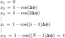 (8-39)
These definitions allow us to prepare the following Step-by-step to calculate the geometry of any 4-digit airfoil.
Step 1: Preliminary Values
Decide the thickness ratio, camber, and location of the camber using the variables t, C, and xcamber, respectively. If the thickness ratio is 15%, then t = 0.15. If the camber is 4%, then C = 0.04. If the location of the camber is 40%, then xcamber = 0.4. (These numbers represent the NACA 4415 airfoil.)
Step 2: Airfoil Resolution
Decide how many x-values (and thus y-values) to include in the analysis. Here, let’s call that value N (e.g. N = 100 for 100 points).
Step 3: Prepare Ordinate Table
Tabulate the x-ordinates along the unit chord using the cosine scheme where Δϕ is calculated using Equation (8-38). These values should range from 0 to 1, where x = 0 represents the leading edge and x = 1 the trailing edge.
Step 4: Calculate Thickness
Calculate the thickness of the upper and lower surfaces of the airfoil for each x-value, from:
![]() (8-40)
(8-40)
Step 5: Compute the y-value for the Mean-line
The next step involves computing the y-value of the mean-line for each x, which we call yc. This depends on whether x is larger or smaller than the location of the camber and is given by:
Step 6: Calculate the Slope of the Mean-line
Calculate the slope of the mean-line at the point:
Step 7: Calculate the Ordinate Rotation Angle
Calculate the angle θ as follows:
![]() (8-45)
(8-45)
Step 8: Calculate the Upper and Lower Ordinates
Calculate the upper and lower surface ordinates as follows:
![]() (8-46)
(8-46)
Generation of the NACA 4415 – an Example Implementation
This procedure has been implemented as shown in Figure 8-27, for a NACA 4415 airfoil, using N = 30. More points should be used for a serious design project. Let’s perform a sample calculation for the row with ID number 10 or i = 10 (see the highlighted row in the figure). Beginning with column 2, we calculate the cumulative sector angle ϕ based on Equation (8-38) as follows:
![]()
where Δϕ = 3.1034° and i is the index in the first column (titled “ID”).
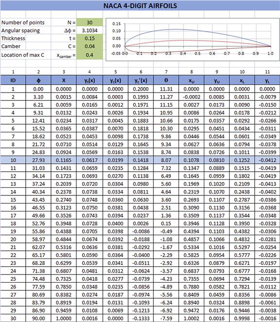
Column 3 is the x-value using the cosine scheme, calculated using Equation (8-39):
![]()
Column 4 is the thickness, calculated using Equation (8-40):
![]()
Column 5 is the y-value of the mean-line, calculated using Equation (8-41) since x10 < xcamber:
![]()
Column 6 is the slope of the mean-line, calculated using Equation (8-43) since x10 < xcamber:
![]()
Column 7 is the slope of the mean-line in degrees, calculated using Equation (8-45):
![]()
The remaining columns 8–12 are calculated using Equation (8-46). The spreadsheet can be used to determine the geometry of any NACA four-digit airfoil by simply changing the thickness fraction, camber, and the location of the camber.
8.2.3 NACA Five-digit Airfoils
The NACA five-digit airfoils can be traced to the work of Jacobs and followed the development of the four-digit airfoils. The thickness distribution was identical to that of the four-digit series; however, the mean-line was modified to place the “maximum camber unusually far forward,” to quote the title of NACA-TR-537 [21], which details their investigation. The investigation of these airfoils followed the revelation that the forward position of the maximum camber resulted in an increase of the maximum lift [22]. The 5-series airfoils were designed to generate a high maximum lift coefficient, and low drag and pitching moment coefficients. A family of the five-digit series features a reflexed camber to provide a zero Cm but have seen limited use. A typical NACA 5-digit airfoil is shown in Figure 8-28.
The reader is directed to Section 8.2.10, Famous airfoils, which discusses a few issues affecting a member of this family of airfoils, the NACA 23012 airfoil. As shown in Refs [21,22], these airfoils generally have poor stall characteristics because of a sharp loss in lift immediately after stall and, although generating impressive maximum lift and minimum drag, this is a very serious drawback.
Applications
The airfoils are widely used in GA aircraft, commuters, and business jets, where they are used for wings. Among aircraft using five-digit airfoils are a number of models manufactured by Beechcraft.
Numbering System
Per Ref. [21], “the first digit is used to designate the relative magnitude of the camber.” NACA R-824 [23] adds that “the first digit indicates the amount of camber in terms of the relative magnitude of the design lift coefficient; the design lift coefficient in tenths is thus three-halves of the first integer.” Thus, considering the airfoil NACA 23012, the 2 means that the maximum camber height is 2%/100 = 0.02 and the design lift coefficient is (2/10)·(3/2) = 0.3. The second digit, when divided by 20, would give the chordwise location of the maximum camber (0.15). The third digit is ‘0’ for normal camber and ‘1’ for reflexed airfoils like those used for flying wings. The last two digits represent the thickness of the airfoil (0.12 or 12%). Using this nomenclature, the various members of the family of five-digit airfoils would be represented as shown in Table 8-2.

Computation of Airfoil Ordinates
This information can now be used to mathematically compute the shape of any 5-digit airfoil as shown in the Step-by-step below:
Step 1: Preliminary Values
Decide the thickness ratio, camber, and location of the maximum camber using the variables t, C, and xcamber, respectively. If the thickness ratio is 12%, then t = 0.12. If the camber is 2%, then C = 0.02. If the location of the maximum camber is 15%, then xcamber = 0.15. (These numbers represent the NACA 23012 airfoil.)
Step 2: Airfoil Resolution
Decide how many x-values (and thus y-values) to include in the analysis. Here, let’s call that value N (e.g. N = 100 for 100 points).
Step 3: Prepare Ordinate Table
Tabulate the x-ordinates along the unit chord using the cosine scheme where Δϕ is calculated using Equation (8-38). These values should range from 0 to 1, where x = 0 represents the leading edge and x = 1 the trailing edge.
Step 4: Calculate Thickness
Calculate the thickness of the upper and lower surfaces of the airfoil for each x-value, using Equation (8-40), repeated here for convenience:
![]() (8-40)
(8-40)
Step 5: Compute the y-value for the Mean-line
The next step involves computing the y-value of the mean-line for each x, which we call yc. This depends on whether x is larger or smaller than the location of the camber and is given by:
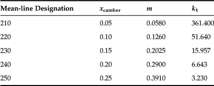
Step 6: Calculate the Slope of the Mean-line
Calculate the slope of the mean-line at the point using Equations (8-43) and (8-44), also repeated for convenience:
Step 8: Calculate the Upper and Lower Ordinates
Calculate the upper and lower surface ordinates using Equations (8-46):
![]() (8-46)
(8-46)
It is of interest to note that it is possible to calculate the constant m and k1 for any position of the xcamber using the following expressions, which are obtained through simple curvefit to the data in the table in Step 5:
![]() (8-49)
(8-49)
Note that the equation for k1 did not have a perfect correlation like the one for m. For this reason, values of k1 calculated using Equation (8-49) will differ slightly from those in the table, although the accuracy gives acceptable results. This allows the evaluation of alternative versions of the five-digit series airfoils. Corresponding values for m and k1 for reflexed airfoils (211, 221, etc.) are given in Ref. [21].
This procedure has been implemented as shown in Figure 8-29, for a NACA 23012 airfoil, using N = 30. More points should be used for a serious design project. In fact, the primary difference between this scheme and the one for the four-digit airfoil is the determination of m, k1, and then the calculation of the mean-line. Here m = 0.2025, k1 = 15.957, although it is calculated using Equation (8-49) A sample calculation for the row with ID number 10 or i = 10 (see the highlighted row in the figure) is provided. First, columns 2 and 3 are identical to the previous approach. The thickness calculated in column 4 also uses Equation (8-40), but this time it yields 0.0494.
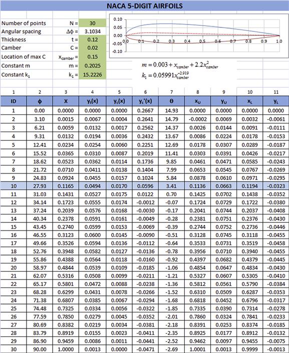
Column 5 is the y-value of the mean-line, calculated using Equation (8-47) since x10 < xcamber:
![]()
Column 6 is the slope of the mean-line, calculated using Equation (8-43) since x10 < xcamber:
![]()
Column 7 is the slope of the mean-line in degrees, calculated using Equation (8-45):
![]()
The remaining columns 8–12 are calculated using Equation (8-46). The spreadsheet can be used to determine the geometry of any NACA 5-digit airfoil by simply changing the appropriate parameters.
8.2.4 NACA 1-series Airfoils
The 1-series airfoils were designed in the late 1930s after the four- and five-digit series (which explains the order of the airfoils in this presentation). The geometry was based on thin airfoil theory rather than on specifying the location of the max camber and then applying the thickness distribution of the preceding families of airfoils. They marked the first time inverse airfoil design was put to use. Theses airfoils are primarily used for propellers, as they prevent the formation of large pressure peaks that are detrimental to airfoils near supersonic airspeeds. It is primarily the 16-version of the 1-series airfoils that is mostly used, so these are sometimes referred to as the 16-series rather than the latter. Reference [24] presents a computer code to help develop ordinates for NACA 16-series airfoils. A typical NACA 1-series airfoil is shown in Figure 8-30.
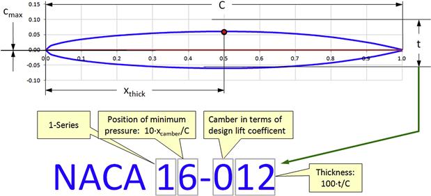
Applications
Widely used for aircraft and ship propellers.
Numbering System
Typical 1-series airfoils are designated by a five-digit number such as NACA 16-212. The first integer ‘1’ represents the series. The second digit ‘6’ denotes the distance in tenths to the chordwise location of the minimum pressure when the symmetrical airfoil is at zero lift (60%). The first number following the dash ‘2’ is the amount of camber in terms of the design lift coefficient in tenths (0.2). The final two digits ‘12’ represent the thickness of the airfoil (0.12 or 12%).
8.2.5 NACA 6-series Airfoils
The 6-series airfoils represent a family of airfoils that were designed to sustain the laminar boundary layer over a larger portion of the chord than the four- or five-digit series. This was accomplished by delaying the development of an adverse pressure gradient by bringing the thickness of the airfoil as far aft as possible before an inevitable separation would ensue. The thickness of these airfoils was developed using exact airfoil theory and for that reason no simple formulation is available in the literature like that for the four- and five-digit airfoils. However, their camber, which is based on thin-airfoil theory, is described in NACA R-824 [23].
A sub-family of the NACA 6-series is called the 6A-series airfoils. They were designed to eliminate the trailing edge cusp associated with the former, which posed great difficulties in their fabrication [25]. For instance, conventional construction methods that require folding aluminum sheet to form such a trailing edge results in geometry far too tight to accommodate supporting ribs in the trailing edge. As a consequence, the trailing edge is unsupported and at higher angles-of-attack it can flex, effectively modifying the airfoil. Reference [26] presents a Fortran IV code to develop the ordinates of NACA 6-series airfoils. Note that Ref. [27] presents an updated version of the code that is more portable between machines.
Applications
The airfoils are widely used for aircraft ranging from WWII era fighters to high-performance GA aircraft, business jets, and military trainers.
Numbering System
The NACA 6-series airfoils (Figure 8-31) feature a six-digit designation with an indicator of the mean-line used. For instance, the designation for the airfoil NACA 653-415, a = 0.5, the ‘6’ refers to the 6-series airfoils, ‘5’ denotes the chordwise location of the maximum camber in tenths of the chord (50%). The subscript ‘3’ gives the range of lift coefficients below and above the design lift coefficient in which favorable pressure gradients exists on both surfaces (± 0.3). The ‘4’ following the dash indicates the design lift coefficient in tenths (0.4). In this way, the particular airfoil is expected to sustain laminar flow for lift coefficients ranging from 0.1 to 0.7 (i.e. 0.4 ± 0.3). The last two digits indicate the airfoil thickness as percent of the chord (0.15 or 15%). The designation “a = 0.5” refers to the mean-line used, but this is used in the derivation of the ordinates. When a mean-line designation is omitted the default value of a = 1.0 is used.

The airfoil designation has a number of variations. For instance, the above airfoil (NACA 653-415) is sometimes represented as NACA 65(3)-415 or 65,3-415.
The camber line can be a combination of more than one such line and then the design lift coefficient is the sum of all the camber lines used; for instance, the “2” in 218 in the following airfoil designation:
![]()
If the thickness distribution of an airfoil is obtained by linearly increasing or decreasing the ordinates of one of the original thickness distributions, then the airfoil is denoted as shown in the example below:
![]()
Where the number ‘3’ in the parentheses denotes the low-drag range and the ‘18’ denotes the thickness ratio of the original thickness distribution. NACA 6-series airfoils whose thickness ratio is less than 0.12 usually do not have a subscript as their low-drag range is less than 0.1 (meaning the subscript should be a fraction). In this case, the subscript is omitted, as shown below:
![]()
There are other deviations, but an interested reader is directed to Ref. [23] for more details.
8.2.6 NACA 7-series Airfoils
The NACA 7-series airfoils were designed to maximize the extent of laminar flow on the upper and lower surfaces, recognizing the two can be different from each other. A typical NACA 1-series airfoil is shown in Figure 8-32.
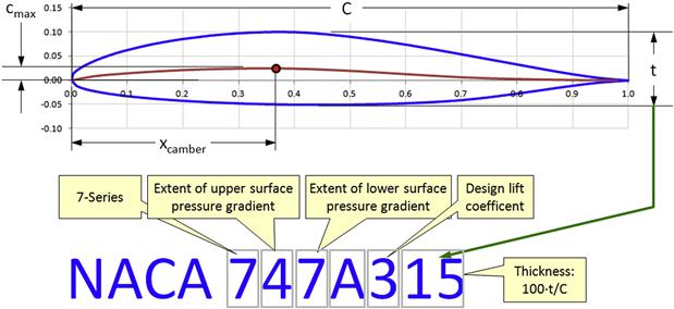
Applications
Not widely used. The University of Illinois at Urbana-Champaign (UIUC) airfoil database indicates five airplane types that use such airfoils; the Brändli BX-2 Cherry, DRS Sentry HP (UAV), Jameson RJJ-1 Gypsy Hawk, MacDonald S-20, and the RFB RW.3-A3 Multoplane.
Numbering System
The NACA 7-series have their own numbering system best explained by considering a typical type: NACA 747A315. The ‘7’ indicates the series number. The ‘4’ indicates the extent of favorable pressure gradient over the upper surface of the airfoil in tenths of the chord length (40%). The next, ‘7’, similarly, indicates the extent of favorable pressure region over the lower surface in tenths of the chord length (70%). This means that as long as the surface qualities are smooth, the laminar boundary layer should extend at least that far aft. The series of three numbers ‘315’ following the letter ‘A’ is identical to that of the 6-series, i.e. ‘3’ is the design lift coefficient (0.3) and ‘15’ is the thickness ratio in hundredths (0.15 or 15%). The intent of the ‘A’ is to distinguish between airfoils that have properties that would lead to an identical digit, but differ in camber or thickness distribution. As an example, another airfoil of the series with an equal coverage of favorable pressure gradients, but with a different camber-line or thickness distribution, would be distinguished from the first one using the serial letter ‘B’. As with the 6-series airfoils, the 7-series also feature camber lines that are the combination of two or more lines.
8.2.7 NACA 8-series Airfoils
In 1949, NACA developed an additional family of airfoils, called the 8-series [28]. These airfoils were developed to prevent the abrupt loss of lift (exemplified in Figure 8-51) near the critical Mach number (see Section 8.3.7, The critical Mach number, Mcrit). These airfoils have not seen much use and were abandoned in favor of Peaky airfoils (see Section 8.2.10, Famous airfoils), which were designed some 10–15 years later. They are really presented here in the interests of completeness.
Applications
No known application.
Numbering System
The numbering system for typical NACA 8-series airfoils is best explained by considering a representative type, e.g. NACA 835A216. The first digit, ‘8’, identifies the series. The second one, ‘3’, denotes the position of the minimum pressure on the upper surface in tenths (0.30). Similarly, the third digit, ‘5’, is the position of the minimum pressure on the lower surface. The letter ‘A’ has an identical function as in the 7-series airfoils, as do the remaining three digits, where the first ‘2’ is the design lift coefficient in tenths (0.2) and the two remaining characters are the airfoil thickness in hundredths (0.16 or 16%).
8.2.8 NACA Airfoils in Summary – Pros and Cons and Comparison of Characteristics
The general advantages and disadvantages of NACA airfoils are summarized in Table 8-4. Also note Figure 8-33 and Figure 8-34, which show typical differences in lift, pitching moment, and drag for the different classes of airfoils.
TABLE 8-4
Pros and Cons of the NACA Airfoils Presented
| Pros | Cons | |
| Four-digit | Generally thick airfoils with benign stall characteristics. Insensitive to non-smooth surfaces. Center of pressure has limited movement over a wider range of AOA. | Relatively low Clmax and high Cdmin and |Cm|. |
| Five-digit | High Clmax and relatively low Cdmin and |Cm|. Insensitive to non-smooth surfaces. | Abrupt stall characteristics. |
| 16-Series | Prevents high pressure peaks that lead to detrimental performance near M = 1. | Low Clmax |
| 6-Series | Relatively high Clmax and low Cdmin. Sustains extensive laminar flow if surface is smooth and forms a drag bucket. Relatively thick. | Sensitive to non-smooth surfaces. High |Cm|. Higher drag outside the drag bucket than that of the 4- and 5-digit airfoils. Some have poor stall characteristics. |
| 7-Series | Low Cdmin. Sustains extensive laminar flow if surface is smooth and forms a drag bucket. Lower |Cm| than the 6-series. Some display good stall characteristics. | Sensitive to non-smooth surfaces. Low Clmax. |
| 8-Series | N/A | N/A |
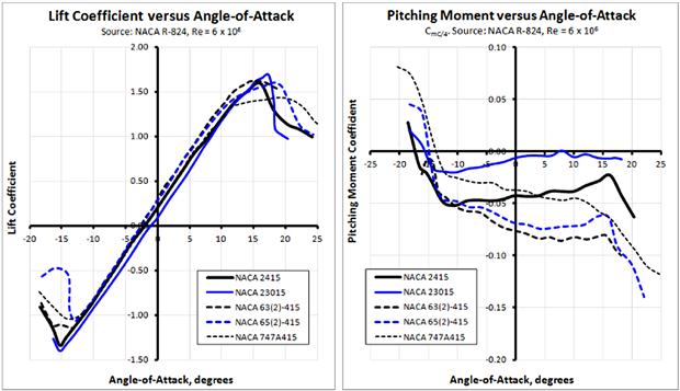
FIGURE 8-33 Lift curve and pitching moment characteristics of selected NACA series airfoils. (from Ref. [23])

FIGURE 8-34 Drag polars of selected NACA series airfoils. (from Ref. [23])
8.2.9 Properties of Selected NACA Airfoils
A substantial amount of aerodynamic data exists on NACA airfoils, as has already been pointed out in the preceding sections. Table 8-5 shows a number of properties for selected airfoils. Note that the widths of the shaded bars in the columns denoted by Clmax, Clα, Cdmin, and Cm ac denote the most favorable values. Thus the widest bar in the Clmax column shows the highest Clmax. The shortest bar in the Cdmin column denotes the lowest values of the drag coefficient, and so on.
TABLE 8-5
Properties of Selected NACA Airfoils (More shading indicates more desirable characteristics)
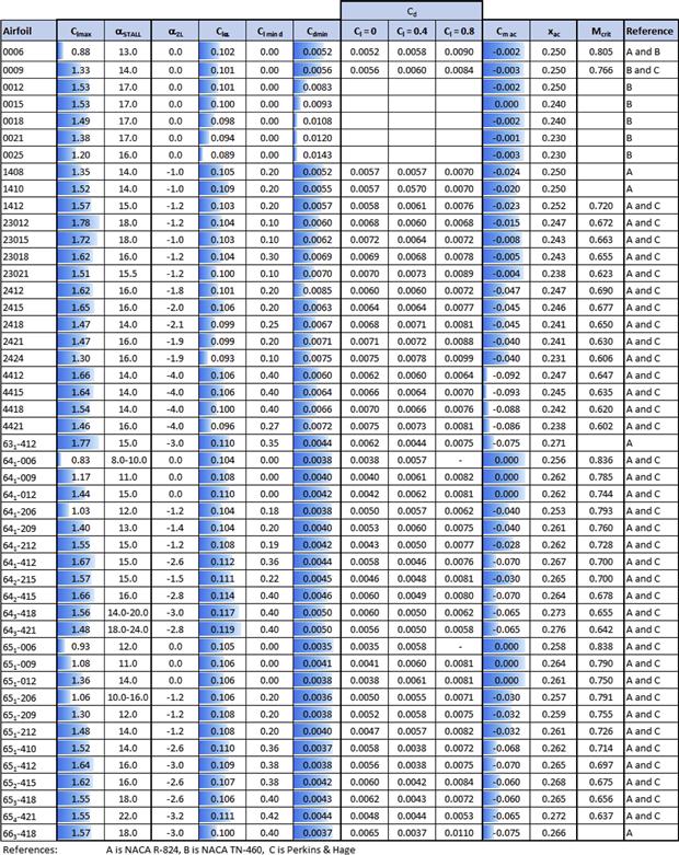
This allows the table to be further manipulated and sorted by the highest Clmax or the lowest Cdmin. This is shown in Tables 8-6 and 8-7. The reader should be reminded that these only apply to the airfoils shown in Table 8-5.
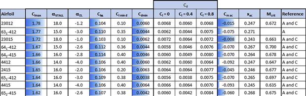
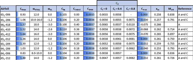
8.2.10 Famous Airfoils
CLARK Y
The Clark Y airfoil (see Figure 8-35) is famous for being one of the most widely used airfoils in the history of aviation, although its use is mostly in airplanes designed before World War II. It is named after Colonel Virginius E. Clark (1886–1948), who designed many airfoils around the time of World War I. The Clark Y airfoil, in particular, was designed in 1922. One of its distinguishing features is the flat lower surface, which extends from 30% chord to the trailing edge. The aerodynamic properties of the Clark Y airfoil can be found in NACA R-502 [29]. Among famous aircraft types that feature this airfoil are the Ryan NYP Spirit of St. Louis, flown by Charles Lindbergh across the Atlantic in 1927; the Lockheed Vega, flown by Amelia Earhart across the Atlantic; and Wiley Post (which he named “Winnie Mae”) twice around the globe. The University of Illinois at Urbana-Champaign (UIUC) airfoil database cites this airfoil 493 times for the 7420 aircraft type instances.
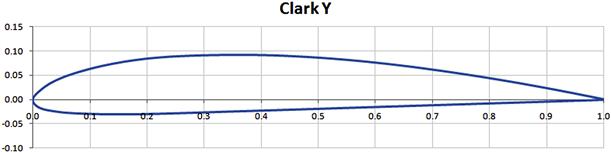
USA-35B
The USA series of airfoils was designed by engineers of the United States Army (USA) in the era before 1920. The USA35B (see Figure 8-36) is the best known. It is a flat-bottomed airfoil used in many well-known aircraft, especially in a line of aircraft made by Piper Aircraft, such as the Piper J-3 Cub, PA-25 Pawnee, PA-23 Apache and Aztec twin-engine aircraft. Like the Clark Y airfoil, it features a substantial camber and generates a high maximum lift coefficient and gentle entry into the post-stall region, but also high drag.
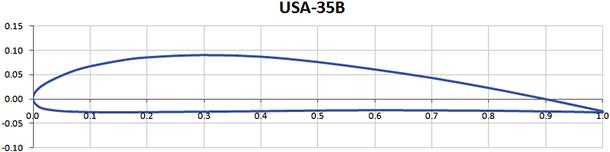
NACA 23012
The NACA four-digit airfoils were developed in the 1930s. This work led to the development of the 23-thousand series airfoils. One of the best known of those airfoils is the NACA 23012 (see Figure 8-37), which is used in a number of aircraft. The UIUC airfoil database cites the airfoil 397 times for the 7420 aircraft type instances, including very common aircraft such as Beech’s Bonanza and B1900 Airliner, just to name a few. It is also featured on the twin-engine Britten-Norman BN-2 Islander, Cessna 208 Caravan and even the Citation jet.
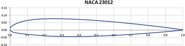
Research on the lift and drag properties of the symmetrical four-digit NACA airfoils showed that while the drag was quite small, the same could be said of the maximum lift. It was proposed that the maximum lift could be improved by introducing a small camber to the airfoil. This was accomplished by simply deflecting the forward part of the leading edge. As can be seen in Figure 8-38, the 23012 airfoil is effectively a NACA 0012 airfoil whose forward 15% has been deflected leading edge down. This new airfoil showed great promise in wind tunnel testing, offering a low Cdmin, very high Clmax, and low Cm, all are great properties that make the airfoil very tempting for the aircraft designer. However, what was less touted in the NACA literature was the abruptness of its stall. And this is a serious problem. In fact, it is not just the NACA 23012 that poses such problems, but a host of airplanes that feature a root/tip combination of 23015/23009 and similar.
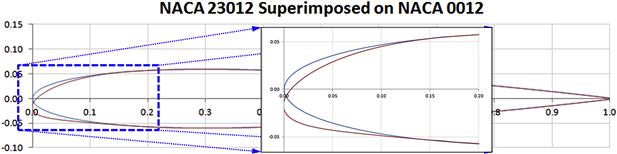
FIGURE 8-38 The NACA 23012 superimposed on the NACA 0012 airfoil reveals the only difference between the two is from the leading edge to 0.15C. A closer look at the leading edge of the two airfoils shows how the leading edge of the NACA 23012 airfoil.
As stated in Section 8.1.11, Airfoil stall characteristics, a leading-edge separation bubble may form on airfoils whose thickness-to-chord ratio is 12% or less. Compounding this issue on the NACA 230XX series airfoil is the nature of its geometry: the leading edge deflection at 15% chord. This introduces a sharp discontinuity in the curvature of the airfoils that may also contribute to the formation of the separation bubble [30]. As the AOA of the airfoil is increased, the airflow will reattach behind the bubble (see schematic to the left in Figure 8-39) and separate again at the trailing edge. With further increase of AOA the second separation point will continue to move forward, eventually and suddenly combining with the leading-edge separation bubble. When this happens, there will be an abrupt and large drop in the lift coefficient. This is clearly visible as the sharp drop in Figure 8-39, from the wind tunnel test data presented in NACA TR-537 [31].
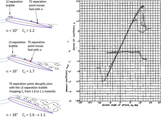
FIGURE 8-39 Data from NACA R-537 for the NACA 23012 airfoil. It clearly displays the sharp drop in the lift coefficient at stall.
Once featured on a wing, fabrication differences between the two wing halves on either side of the plane of symmetry will result in a high probability that one wing will stall (abruptly) before the other. In other words, an uncontrollable roll-off at stall is a very plausible scenario the designer should be strongly aware of. And while it is certainly possible to “beat” this detrimental stall behavior into submission with adequate wing washout and stall strips, this is likely to take extra development time and cost, making the series of airfoils something the aircraft designer should stay away from. There are multiple other options at the disposal to the designer which offer similar favorable properties but with far more benign stall characteristics.
GA(W)-1 or LS(1)-0417
The GA(W)-1 (see Figure 8-40) was designed in 1972 specifically for GA aircraft using computational fluid dynamics by Robert T. Whitcomb and associates at the NASA Langley Research Center [32]. Details of its characteristics can be found in the report NASA TN D-7428 [33]. It is also known as NASA/Langley/Whitcomb LS(1)-0417. The report tested the airfoils at Reynolds numbers ranging from 2 × 10⁶ to 20 × 106 and Mach numbers ranging from 0.15 to 0.28 and demonstrated CLmax ranging from 1.6 to 2.0. A selection of lift-to-drag ratios between 65–85 were obtained at a climb lift coefficient of 1.0. These characteristics appeared very promising and the airfoil was featured on at least two aircraft designs from the 1970s: the Piper PA-38 Tomahawk and Beechcraft 77 Skipper. Other aircraft using the airfoil are the cancelled American Aviation Hustler, the Edgley Optica, and the cancelled military trainer Fairchild T-46 Eaglet.
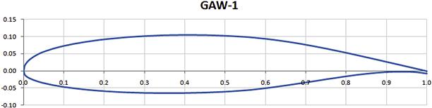
Among other favorable characteristics is the structural depth offered by its thickness-to-chord ratio of 17%. This provides the aircraft with ample volume for fuel and should result in a lighter wing structure. The cusp (reflexed curvature) near the trailing edge of the airfoil usually presents an issue when using NLF airfoils, as it results in a thin trailing thickness that makes it practically impossible to fit ribs that extend to the trailing edge. The last 30% of the chord is usually allotted to control surfaces and usually these are constructed using conventional stressed skin aluminum construction. The cusp will then require ribs whose flanges must be curved, which requires costly tooling to fabricate. If the control surfaces are built using composite materials the cusp can be accommodated, although such surfaces usually end up being heavier than if they were made from aluminum. Overall, the cusp presents a hard detail in real production environment and sometimes forces the manufacturer to modify the geometry by making the control surfaces flat-bottomed.
Davis Wing Airfoil
The Davis wing is the topic of discussion in online Appendix C1.5.1, The Davis wing, but it stood for a wing design philosophy used for many military aircraft, of which the Consolidated B-24 Liberator is probably the best known. The airfoil, which was inspired by what, at the time, was thought to be the shape of a teardrop (see Figure 8-41), had a number of interesting characteristics, most prominent of which was low drag and high lift. The airfoil was evaluated in NACA WR-L-677 [34]. An Xfoil analysis of the airfoil at a Reynolds number of 9 × 10⁶ matches the experiment reasonably well and indicates it has many interesting properties. Among those are gentle stall characteristics, LDmax in excess of 160, and a Clmind of 0.65 (suitable for a lumbering heavy transport aircraft). Xfoil under-predicts the Clmax of about 1.35 versus 1.4 from experiment, but the Clmind between prediction and experiment match well.

“Peaky” Airfoils
A peaky airfoil is a name used for airfoils that were designed in the 1960s for use in aircraft operating in the transonic range (see Figure 8-42). When conventional airfoils accelerate to high subsonic airspeeds a shockwave begins to form well below Mach 1. This takes place as the speed of air flowing around the airfoil locally reaches and exceeds the speed of sound on the airfoil. As soon as shocks begin to form in the flow there will be a sharp rise in the drag of the airfoils, as shown in Figure 8-50. The airspeed at which this drag rise begins is the critical Mach number (see Section 8.3.7, The critical Mach number, Mcrit). Mcrit for typical NACA four-digit or five-digit airfoils may be as low as a hair over Mach 0.6, depending on thickness. This renders them impractical for use in high-speed aircraft. A strong shock wave will form on such airfoils, greatly increasing their drag and reducing their lift, and may even introduce aeroelastic problems to the vehicle [35]. It is possible to delay these effects by increasing the sweep of the wing, but eventually they are inescapable.
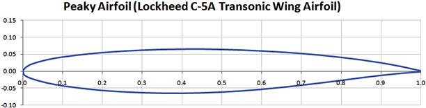
As soon as the shock forms, the center of lift of the airfoil moves from approximately the quarter-chord to the mid-chord, further compounding the issue by substantially increasing stability. Additionally, the shock will induce separation, which thickens the wake aft of the shock (see Figure 8-43), increasing the drag further [36]. What follows is a complex interaction of the movement of the upper and lower shockwaves that ultimately results in a drastic drop in the lift coefficient being produced, causing a shock-stall.

FIGURE 8-43 A Schlieren photograph of the flow past a 10% RAE 102 airfoil. Visible is the severe separation at the foot of the upper-surface shock, as well as an lower-surface shock. AOA is 2° and M = 0.88. (Photo from Ref. [36])
Research on such high-speed effects began early, or in the 1940s, but serious work on modifying airfoils began in 1955 with the pioneering work of H. H. Pearcey, who tried to experimentally obtain “an essentially shock-free flow” [37]. Pearcey showed that by reshaping the leading edge of an airfoil it was possible to weaken the shock. The process was to allow the flow to expand rapidly from the stagnation point and become supersonic in the leading edge area. This would form a series of compression shock waves that slowed the local Mach number, so the final shock wave was substantially weakened [38]. Less drag was one important benefit from this change. It was thought the modified airfoils would be capable of weakening the shock for maximum local Mach numbers as high as 1.4. The resulting pressure distribution has a prominent pressure peak near the leading edge and was described as being peaky. The airfoil has a relatively flat upper surface, which necessitates a cusp in the trailing edge to improve its lift generation.
Experience in using peaky airfoils on combat aircraft has revealed that high-speed, high-g maneuvers (which call for high AOA) result in the formation of significant shock strength that may cause sudden loss of lift. When introduced to the Hawker-Siddeley Kestrel FGA.1, the prototype of the production Hawker-Siddeley Harrier, this shock would occur above Mach 0.8, causing a serious wing-rocking at an AOA where a gentle buffet would be expected [38].
Supercritical Airfoils
Supercritical airfoils are often referred to as one of the three major contributions to aviation made by the famous aerodynamicist Richard T. Whitcomb (1921–2009), whom many historians of aviation call the most distinguished alumnus of the NASA Langley Research Center. His other two contributions being the area-rule and the winglet.
Like the peaky airfoils, supercritical airfoils are intended for high-speed aircraft. They feature a large radius (blunt) leading edge, considerably flatter upper surface than the peaky airfoils, and a significant cusp near the trailing edge (see Figure 8-44). The blunt leading edge softens the suction peak of the smaller radius peaky airfoil. The flatter top surface helps keep down the local Mach number and keeps down adverse pressure gradients. The cusp was introduced to help generate lift without lowering Mcrit by forming a high-pressure region under the airfoil.
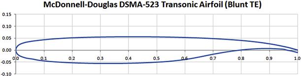
FIGURE 8-44 A transonic blunt TE airfoil developed by McDonnell-Douglas under the designation DSMA-523.
The characteristics of supercritical airfoils can be summarized as follows: (1) the drag rise Mach number, Mcrit, is substantially higher than for more conventional airfoils. As an example, at a section lift coefficient of 0.65, the Mcrit of one such airfoil is 0.79, which compares very favorably to the 0.67 of a NACA 64A-series airfoil of an equal thickness ratio [39]. (2) The section pitching moment coefficient for supercritical airfoils is substantially more negative than for conventional airfoils. This is caused by the high-pressure region that forms at the lower surface due to the cusp. (3) The supercritical airfoil also increases Mcrit at off-design section lift coefficients. (4) The airfoil also increases the maximum lift coefficient at high subsonic Mach numbers.
Wing design that uses supercritical airfoils offers many advantages to a high-speed aircraft. First, and as has already been stated, is the increase in Mcrit for a given thickness and wing sweep. Second, their thickness offers structural depth and volume for fuel. Third, they allow the designer to reduce the wing sweep, which offers a host of benefits. Among those are improvements in low-speed characteristics and performance capabilities.
Joukowski Airfoils
Joukowski airfoils are a much more clever mathematical tool used to demonstrate aerodynamic theory than a practical solution to aircraft design. The airfoils are named after the Russian scientist Nikolay Yegorovich Joukowsky (sometimes spelt Zhukovsky, 1847–1921), who is also the originator of the circulation theorem (see Section 8.1.8, The generation of lift). The airfoils are generated in conformance with the transformation of a circle on to the complex plane, using the complex number ζ:
![]() (8-50)
(8-50)
Consider the complex number ζ to be given by ![]() . Inserting this into Equation (8-50) and manipulating yields the two spatial variables x and y that are given by the following relation:
. Inserting this into Equation (8-50) and manipulating yields the two spatial variables x and y that are given by the following relation:
![]() (8-51)
(8-51)
By varying the values of a and b between −1 and 1 (e.g. try a = −0.1 and b = 0.1) the shape of the airfoil can be modified (see Figure 8-45). Then, using elementary flow concepts, such as uniform flow, sources, sinks, and vortex flow, airflow around the resulting airfoil can be simulated. Joukowski airfoils are a subject in most texts on theoretical aerodynamics, although they are rarely used on actual aircraft. In fact, the UIUC airfoil database indicates five instances, all of them sailplanes (the Schempp-Hirth Gö-4 III Goevier, Schleicher ASK 14, ASK 16, ASK 18, and Schleicher Ka-6 Rhönsegler).
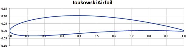
Liebeck Airfoils
The unconventionally shaped airfoil shown in Figure 8-46 is named after Dr. Robert Liebeck, who was one of the first to try and find out what sort of “airfoil-shaped” geometry would yield the highest possible Clmax. The answer is the shape devised by Dr. Liebeck, which is remarkable for achieving the highest lift-to-drag ratio of any airfoil. The airfoils are designed to utilize Stratford distribution (see Section 8.1.6, Chordwise pressure distribution) and achieve an L/D ratio in excess of 600. The airfoils are intended for low Reynolds number applications. There is a large amount of scientific literature available that investigates the properties of these airfoils.
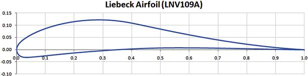
8.3 The Force and Moment Characteristics of the Airfoil
As discussed in Section 8.1.3, Representation of forces and moments, the lift, drag, and pitching moment generated by the airfoil is almost always converted into a dimensionless coefficient form. The primary advantage of this is transferability. Transferability means that if the coefficients are known for a particular airfoil geometry, they can be used to extract forces and moments for any other size of the airfoil, airspeed and atmospheric conditions. These coefficients are defined as shown below
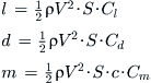 (8-52)
where
m = pitching moment, in N·m or ft·lbf
S = reference area, typically wing area, in m2 or ft2
Cl = non-dimensional lift coefficient that relates AOA to the lift force
Cd = non-dimensional drag coefficient that relates AOA to the drag force
Cm = non-dimensional pitching moment coefficient that relates AOA to the pitching moment
8.3.1 The Effect of Camber
Introducing positive (or negative) camber to an airfoil will have a profound effect on its lift curve and drag polar. These are illustrated in Figure 8-47. A positive camber will shift the lift curve to the left and up, resulting in a higher Clmax, and introduce a negative zero lift angle (αZL) and a positive value to the lift coefficient at α = 0° (Clo). The opposite happens if a negative camber is introduced.
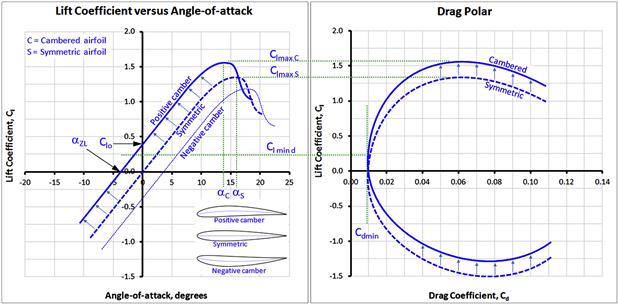
The camber will also change the drag polar. If the camber is modest, as is usual for most airfoils, the change will primarily be in the shifting of the drag polar (see Figure 8-47). This change introduces a new variable, Clmind, which is the value of the lift coefficient where the airfoil’s minimum drag coefficient, Cdmin, occurs. Cdmin for a symmetrical airfoil is at Cl = 0. If the change in the camber is large (as happens when flaps are deflected) the shape of the drag polar will change and be shifted to a higher Cdmin as well.
8.3.2 The Two-dimensional Lift Curve
The lift coefficient relates the AOA to the lift force. If the lift force is known at a specific airspeed the lift coefficient can be calculated from:
![]() (8-53)
(8-53)
In the linear region, at low AOA, the lift coefficient can be written as a function of AOA as shown below:
![]() (8-54)
(8-54)
Equation (8-54) allows the AOA corresponding t o a specific lift coefficient to be determined, provided the lift curve slope known:
![]() (8-55)
(8-55)
Equation (8-55) is only applicable in the linear region, like the one shown in Figure 8-3.
8.3.3 The Maximum Lift Coefficient, Clmax
Standard lift curve graphs, which plot the variation of the lift coefficient with AOA, usually show a very distinct peak (e.g. see Figure 8-39). This peak is the maximum lift coefficient and both it and the AOA at which it occurs are of profound importance in the development of any mechanical device that depends on aerodynamic forces.
The shape of the lift curve in this region is of importance as well. Airfoils that display a sharp drop in the lift curve at stall should be avoided for use in aircraft, in particular if benign stall characteristics are being sought.
Maximum Theoretical Lift Coefficient
Questions such as “what is the maximum value of the lift coefficient?” and “what kind of shape yields that value?” are often asked. Answers to these questions are addressed in a classic paper by Smith [3]. Knowing the theoretical limits is important for comparison reasons. It allows efficiency and potential for improvements to be quantified. Figure 8-48 shows a cylinder of diameter d, rotating in a uniform inviscid flow of velocity V, exposed to three values of the circulation, Γ. Since the flow is inviscid it will not separate, but rather flow around the cylinder as shown. While such a flow exists only in the imagination, it is still of considerable importance in aerodynamics. Not only does it show what could be were it not for viscosity, it also allows the aerodynamicist to determine theoretical limits.
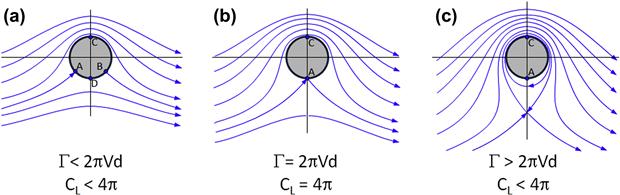
FIGURE 8-48 Potential flow past a circular cylinder drawn for three values of the circulation Γ. (Based on Ref. [46])
Using potential flow theory (PFT), it is possible to simulate airflow around a rotating cylinder by adding the elementary flow functions of uniform and vortex flow. For instance, consider the Figure 8-48(a), which shows two stagnation points, A and B. In Figure 8-48(b), the circulation is strong enough to bring the two stagnation points together, and in (c) it is strong enough to move the stagnation point off the surface. It can be shown using PFT that the circulation required to create the flow in Figure 8-48(b) amounts to 2πVd. For instance see Anderson [40, pp 249–251]. Using Equation (8-26), we can write:
![]()
But it is also possible to write lift using Equation (8-52). Therefore, the lift coefficient, Cl, can be found to equal:
![]()
The corresponding lift coefficients for values of the circulation on either side of 2πVd result in lift coefficients that are less than 4π. A geometry that yields a higher value of the lift coefficients is not known by this author. The value Clmax = 4π can therefore be considered the maximum theoretical lift coefficient.
8.3.4 The effect of Reynolds Number
Figure 8-49 shows how the Reynolds number (Re) affects the airfoil’s lift curve and drag polar. The left graph shows that the slope and intersection of the linear region to the horizontal and vertical axes are unaffected by the Re. However, the higher the Re, the higher is the stall AOA (denoted by α1, α2, and α3), maximum lift coefficient (denoted by CLmax 1, CLmax 2, and CLmax 3), and the point where the slope becomes non-linear. This effect is purely viscous so it is usually estimated through wind-tunnel testing or using viscous computational fluid dynamics flow solvers.
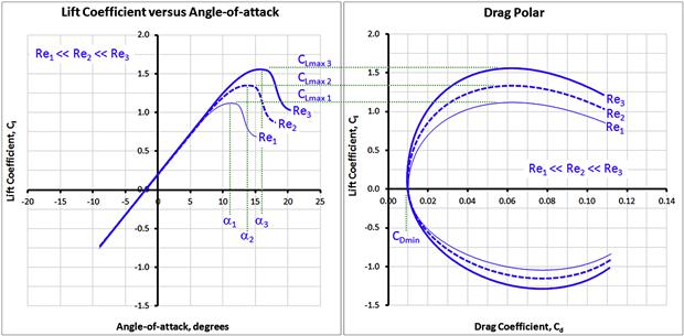
A typical change in the drag polar is shown in the right graph of Figure 8-49. Generally, an increase in Re will not have a large effect on the minimum drag, unless it causes a significant change in the nature of the flow, such as if a laminar boundary layer transitions early into a turbulent one, or as a result of poor surface qualities (e.g. see Section 8.3.13, The effect of leading edge roughness and surface smoothness). On the other hand, it will reduce the Cd elsewhere, thanks to the delayed tendency for flow to separate. For thick airfoils, the high Re delays the forward movement of the trailing edge separation point to a higher AOA, ultimately delaying stall. For this reason, as the Re increases, the drag polar typically gets wider.
8.3.5 Compressibility Effects
Generally, flow can be considered incompressible up to Mach 0.3 and even as high as Mach 0.5. This fact is very convenient to the designer of slow aircraft, as he or she will not have to deal with the added complexity of compressibility. Compressibility requires the introduction of equivalent airspeed (see Section 16.3.2, Airspeeds: instrument, calibrated, equivalent, true, and ground) in addition to modifications that have to be made to the lift, drag and pitching moment coefficients.
Compressibility Effect on Lift
Figure 8-50 shows the effect compressibility has on the airfoil’s lift curve and drag. Compressibility increases the slope of the lift curve. In practice, this means that a smaller AOA is required to generate a given lift coefficient, as is evident from the left graph in Figure 8-50. The designer of GA aircraft is generally only interested in the stall portion of the lift curve at low Mach numbers because such airplanes always stall at low subsonic airspeeds. However, the stall portion is important in fighter aircraft design as such aircraft pull high gs at high airspeeds at AOAs near or exceeding stall.
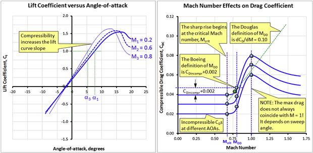
Compressibility Effect on Drag
Compressibility also has important effect on the drag polar (also discussed in Section 15.4.2, The effect of Mach number). The drag coefficient at a given AOA (or Cl) remains relatively constant until the airfoil approaches Mach numbers in the range 0.6 to 0.8. These are called the critical Mach number (see Section 8.3.7, The critical Mach number, Mcrit). Increasing the airspeed further will result in a sudden rise in drag. This is a consequence of a shock forming on the airfoil, as the local velocities exceed the speed of sound. The effect is shown as the sharp rise in the compressible drag coefficient, CDC, in the right graph of Figure 8-50. These are but a part of the intriguing (if not surprising) behavior of fluids near this critical airspeed (M = 1). The so-called drag divergence Mach number, denoted by MDD, is defined after the coefficient has clearly begun to diverge from its incompressible value. Generally, there are two common definitions by two prestigious manufacturers; Boeing and Douglas (which is now a part of Boeing). The Boeing approach defines MDD as the Mach number where the drag coefficient exceeds its incompressible value (CDincompressible in Figure 8-50) by 0.0020. The Douglas approach defined it as the Mach number where the slope dCDc/dM first reaches 0.10 [41]. Section 15.5.12, Drag due to compressibility effects, presents a method to account for this drag.
Compressibility Effect on Lift and Drag Exemplified
Compressibility affects both the section lift coefficient and the section drag coefficient detrimentally at high Mach numbers, as shown in Figure 8-51. These show that at a fixed AOA, there is an abrupt reduction in lift and a sharp rise in drag when the airspeed approaches sonic conditions. This effect happens at the critical Mach number (see Section 8.3.7, The critical Mach number, Mcrit). It is indicative of local airspeeds over the airfoil having exceeded Mach one, forming a normal shockwave that alters the pressure distribution, causing the large deviations seen.
Figure 8-52 shows the effect the Mcrit has on the lift curve slope and the zero AOA lift coefficient. The first observation is that the lift curves at M = 0.4 and 0.6 do not show a large change. However, there is a sharp reduction in the lift curve slope at M = 0.8 (note that the values of Clα and Clo shown are based on the four points at 1° through 4°). This is followed by a slight recovery at the minimum value of the lift coefficients, which occurs at a Mach number of 0.87; however, the zero AOA lift is now negative and almost doubled in magnitude. Any airplane featuring this airfoil (NACA 2412) operating at these Mach numbers would suffer serious stability issues.
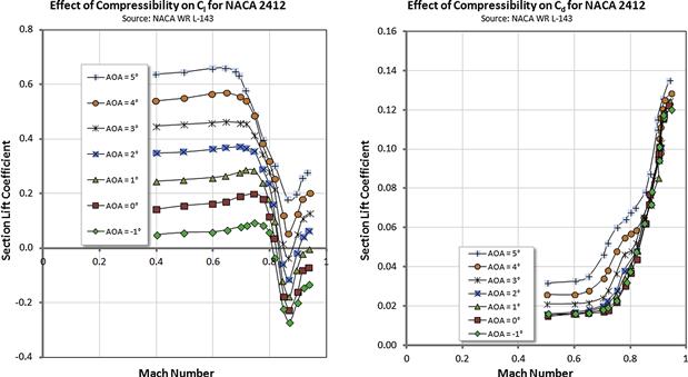
FIGURE 8-51 The effect of Mach number on the lift and drag coefficient of a NACA 2412 airfoil. (Reproduced from Ref. [47].)
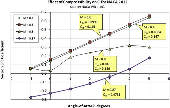
FIGURE 8-52 The effect of Mach number on the lift curve of the NACA 2412 airfoil. The lift curve slope and the lift at zero AOA are shown in the bullets. (Based on analysis using data from Ref. [47])
Compressibility Effect on Pitching Moment
Compressibility has a major impact on the behavior of airfoils and wings at high Mach numbers. It is appropriate to discuss both at the same time. This is shown schematically in Figure 8-53 for a hypothetical aircraft trimmed at M = 0.5. It is of interest to consider the effect in terms of the pitch stability, denoted by Cmα, and stick force, which is the force the pilot must exert in order to control the airplane longitudinally. Of course the graph would be different for other aircraft, CG locations, control system, airfoil types, trim points, and so on. However, considering these at the moment is not necessary to make the following point. As will be discussed in Chapter 11, The anatomy of the tail, static stability of aircraft requires Cmα to be negative (here, for the example aircraft, it is near −1.0 at low Mach numbers. This means that at low airspeeds, the pilot must pull on the yoke (or stick or column) in order to slow down further. Alternatively, he or she must push in order to fly at Mach numbers higher than 0.5.

With respect to the airfoil, as the far-field airspeed increases, a shock-wave begins to form and change the pressure distribution over the wing. The airplane has entered the transonic region. The effect of the shock-wave depends on where on the wing it forms first (inboard, midspan, outboard) and grows with further increase in the airspeed. It is possible to experience a number of different scenarios, besides the one shown in Figure 8-53. The bottom line is that once a given airspeed is exceeded, the pitch stability and stick force will rise rapidly. This is caused by the center of pressure moving from approximately the quarter-chord to the mid-chord. The effect is akin to the CG being moved forward by that amount at subsonic speeds. If the airplane has not been designed for this, it is possible that the magnitude of the stick force will render the airplane uncontrollable – it will enter a dive (recall the moment tends to point the nose down), which will increase the airspeed further, and from which it may not recover.
8.3.6 Compressibility Modeling
The following methods are commonly used to account for the impact of compressibility on pressure coefficients:
Prandtl-Glauert [42]:
![]() (8-56)
(8-56)
 (8-57)
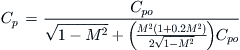 (8-58)
Frankl-Voishel correction for skin friction drag:
![]() (8-59)
(8-59)
while compressibility effects can be included with the lift and moment coefficients as follows (here using the Prandtl-Glauert model):
![]() (8-60)
(8-60)
![]() (8-61)
(8-61)
where the subscripts ‘0’ refer to the incompressible values. The same correction does not hold for the drag coefficient, as it incorporates skin friction as well as pressure drag and will give erroneous results.
8.3.7 The Critical Mach Number, Mcrit
Consider the airfoil (or some arbitrary body) immersed in fluid flow as shown in Figure 8-54. The presence of the body will cause the fluid to accelerate over it, resulting in local speeds that are higher (and lower) in places compared to the far-field speed. In the case of the fluid being air; if the far-field Mach number is denoted by M∞, there will be a different Mach number detected at some arbitrary point A on the body. Then, we define the critical Mach number, Mcrit, as the far-field speed at which the local velocity, anywhere on the body, first achieves M = 1. As has already been discussed, this manifests itself as a sudden rise in the drag of the body.

FIGURE 8-54 An airfoil immersed in airflow with the point of minimum pressure identified as point A.
Typical airfoils begin to experience this phenomenon when the far-field Mach numbers exceed 0.60 to 0.80. The actual value is highly dependent on the geometry of the airfoil, primarily the thickness: Mcrit is much lower for thick airfoils than thin ones. Examples of Mcrit for selected NACA airfoils can be seen in Table 8-5. The Mcrit of airfoils used for high-speed aircraft is normally increased by sweeping the wing forward or aft (see Chapter 9, The anatomy of the wing). Additionally, the effect depends on the AOA. The higher the AOA, the higher are the local airspeeds over the airfoil and this will expedite the onset of the drag rise.
Step-by-step: Determining Mcrit for a Body
The Mcrit can be determined for a body, such as an airfoil or a fuselage, by the application of the following method, based on Anderson [40, pp. 674–679] and Perkins and Hage [43].
Step 1: Establish the Minimum Pressure Coefficient
Using either a theoretical or experimental method determine the low-speed, incompressible minimum pressure coefficient, Cpo, on the body. For airfoils this can be done by any of the freely (and commercially) available computer codes cited in Section 8.1.14, Airfoil design. References [23,44] also list airspeed ratios for a number of NACA airfoils.
Step 2: Select Compressibility Correction Method
Using any of the methods presented with Equations (8-56), (8-57), or (8-58), select the appropriate compressibility correction. Note that Equations (8-57) and (8-58) are generally considered more precise than the Prandtl-Glauert method.
Step 3: Solve to Determine Mcrit
Depending on the compressibility correction method selected, the predicted Mcrit can be found by setting it equal to the following expression, which determines the pressure coefficient required for sonic conditions to prevail at the point of minimum pressure:
![]() (8-62)
(8-62)
An example of this procedure is shown in Figure 8-55, as it is applied to the NASA NLF(1)-0414F airfoil in Figure 8-7.
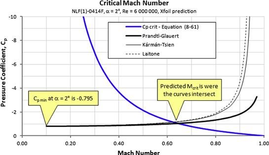
Derivation of Equation (8-62)
As the airspeed (Mach number) increases, the local velocities over an airfoil increase as well. Consider point A on the airfoil in Figure 8-54. Denote the static pressure in the far field with p∞ and at A using pA. Assuming the flow to be isentropic (adiabatic and irreversible) the pressure in the far-field and at A can be related to the total pressure as follows:
Therefore, the pressure at point A can be related to that in the far-field by dividing Equation (i) by (ii) as follows:
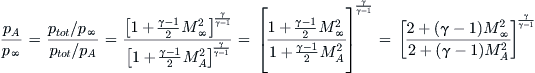 (iii)
(iii)
Of special interest is the case when the airspeed at point A becomes sonic, i.e. MA = 1. Then Equation (iii) can be rewritten as shown below:
![]() (iv)
(iv)
Inserting Equation (iii) into Equation (8-14) and renaming M∞ as Mcrit yields Equation (8-62).
QED
8.3.8 The Effect of Early Flow Separation
Figure 8-56 and Figure 8-57 show the effect early flow separation has on the airfoil’s lift curve and drag polar. This is in fact easy to detect from the lift curve and, thus, the designer reviewing wind tunnel test results should be aware of its nature and not be caught off guard. The effect appears in a similar fashion for two-dimensional airfoils and three-dimensional aircraft as a reduction in the lift curve slope. It can be seen in Figure 8-56 that the slope change is followed by a stall AOA that may be slightly less than what would be expected, and the maximum lift coefficient may be substantially lower. This can cause severe detriments to the low-speed performance of an aircraft, and in the most severe case make a new design impossible to certify. In addition to a smaller CLmax, the slope change will require the airplane to make up for the shallow slope by operating at a higher AOA, with the associated increase in lift-induced drag.

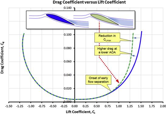
The early separation of two-dimensional bodies, such as airfoils, can be the consequence of the pressure recovery region of the airfoil being too short, the trailing edge region of the airfoil being too steep, or the discontinuity of a surface caused by the presence of a control surface. For efficiency the lift curve should be linear to as high a lift coefficient as possible.
It follows from the coupling of lift and drag that the effect of flow separation impacts the drag polar as well, although it is harder to make out. As shown in Figure 8-57, the effect will narrow the drag polar and deviate from a quadratic approximation (in the absence of a drag bucket) much earlier than what one would expect. As stated above, this means that there will be an unexpected rise in the drag of the aircraft, even at climb AOA, that will lower rate of climb, and reduce optimum operating points, such as endurance and range, which are often achieved at relatively high AOAs.
8.3.9 The Effect of Addition of a Slot or Slats
Figure 8-58 shows the effect of introducing a leading edge slot or slat to an airfoil. The airfoil’s lift curve is modified in an important way as as shown in the figure. Usually, the literature depicts the effect of deploying the slat by showing that the point of stall on the lift curve is extended to a higher AOA and Clmax (or CLmax for three-dimensional geometry). However, two additional effects must be considered as well. The first one is that this is only accurate as long as the deployment changes the overall camber in minute ways only. The second one is that the deployment does not significantly change the chord length of the airfoil. If the shape of the camber changes such that its curvature increases, the lift curve will shift up and left, similar to that of a flap deflection (see Section 8.3.10, The effect of deflecting a flap). If the chord of the airfoil increases as a consequence of deployment, the slope of the lift curve will change as well. In this case, it is most clear to envision the slope change being caused by a larger lift force being converted to a lift coefficient using the original chord-length (or wing area in the case of a three-dimensional wing). If both parameters change noticeably, the resulting lift curve will display a combination of the two effects and not that typically displayed in the literature.
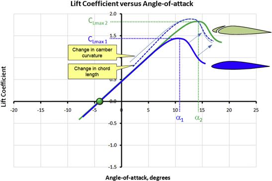
Various leading edge devices are presented in Section 10.2, Leading edge high-lift devices.
8.3.10 The Effect of Deflecting a Flap
Flaps have a significant impact on the aerodynamic characteristics of airfoils. At a given airspeed and AOA, the magnitudes of lift, drag, and pitching moment of an airfoil increase. Figure 8-59 shows the effect of deflecting a flap on a wing’s lift curve. Figure 8-60 show the effect on the drag polar. It is important to keep in mind that deflecting the flap trailing edge down (TED) will move the lift curve up and sideways to the left. This is a consequence of an increase in the airfoil’s camber, but this increases its lift at a given AOA. The opposite takes place if the flap is deflected trailing edge up (TEU). This decambers the airfoil, effectively shifting the lift curve downward and to the right. This means that the stall AOA is shifted as well, to the left or right, depending on the deflection.
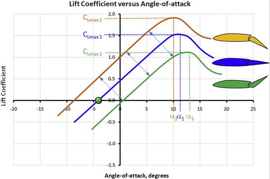

The deflection also affects the drag and increases it regardless of whether the flap is deflected TEU or TED. However, the magnitude and sign of the pitching moment change significantly. Deflecting a flap TEU allows wings to be made statically stable without the use of stabilizing surfaces such as horizontal tails or canards. The magnitude of the change in lift largely depends on the design of the flap, but this is discussed in more detail in Section 10.3, Trailing edge high-lift devices.
8.3.11 The Effect of Cruise Flaps
A cruise flap is a wing control surface whose purpose is to shift the drag polar to the left when deflected (see Figure 8-61). To achieve this effect, the flap must be deflected trailing edge up. As a consequence, the drag characteristics of the aircraft will be significantly affected. The primary effect is that the maximum L/D will now move to a lower value of the lift coefficient. This means that the aircraft will be more efficient at a higher airspeed – and this is favorable because people generally want to travel from A to B fast and efficiently.
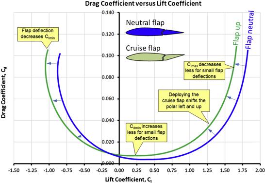
Cruise flaps are a very common feature on sailplanes, where they allow the pilot to fly from thermal to thermal faster to minimize sinking in-between. The total drag coefficient will increase a bit as the polar is shifted to the left and up. However, for low deflection angles, the transverse movement is much larger than the upward one, so there is not a large increase in drag. Cruise flaps will also reduce the Cm as the up-deflected trailing edge will effectively transform the airfoil into a reflexed one. In this way, cruise flaps can reduce trim drag.
Cruise flaps are almost exclusively an extension of the functionality of regular flaps. In other words, the flap control system is designed such that the flap can deflect, say, 5° to 10° trailing edge up in addition to its normal downward deflection. As a consequence, they inflict very limited complexity on its design, although the use of slotted flap types may cause issues due to the upper wing surface extending farther aft (called slot lip).
8.3.12 The Effect of Deploying a Spoiler
A spoiler is a device whose purpose is to increase the drag of the airplane. This is necessary for low-drag airplanes such as sailplanes and jets, to allow them to descend at relatively steep flight path angles. Without such a device, a sleek aircraft would have to descend at a very shallow flight path angle to keep down the airspeed. The resulting landing would be challenging as the airplane would float long distances down the runway before touching down. A spoiler remedies this by allowing for a steeper descent angle at a given airspeed. Devices of this kind are also referred to as an airbrake or speed-brake. Spoilers are very useful for sailplanes, but serve two purposes on jets: to allow a rapid descent from some initial altitude to a lower one; and to ensure the airplane does not bounce after the first touch-down during landing, by “killing” lift. A jet that bounces during landing gets airborne and consumes a lot of runway.
Some people make a distinction between a spoiler and a speed brake, using the term spoiler if the device is deployed from the wing (it “spoils” the lift and increases drag), but using the term speed brake if it is deployed from another part of the aircraft, for instance the fuselage. In this case it only generates drag. The advantage of speed-brakes is that they increase the drag without changing the AOA.
In most cases, the effect of deploying a speed-brake can be approximated by shifting the drag polar upward to a higher Cdmin, while reducing the Clmax. This is shown in Figure 8-62. Note that while the Clmax of the airfoil is decreased significantly due to a “forced” flow separation, the magnitude of the Clmin increases significantly as well (i.e. it becomes even more negative). The effect is similar to using a split flap on an inverted airfoil.
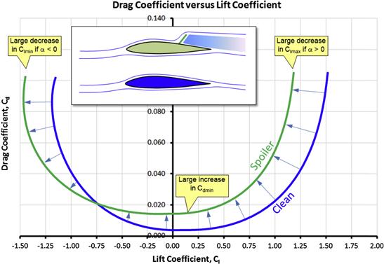
8.3.13 The Effect of Leading Edge Roughness and Surface Smoothness
The quality of lifting surfaces is of great importance and is an effect that was investigated by NACA as early as the late 1930s [45] and showed that surface roughness caused a large increase in drag. It was also shown that smooth surfaces are important even when extensive laminar flow is not to be expected [23]. However, it was also shown that surfaces do not have to be superbly smooth or polished. On the other hand, polishing a surface that is not aerodynamically smooth will reduce its drag. The experimenting showed that 320-grit sandpaper produced acceptable surface smoothness for all aerodynamically smooth surfaces. It also showed that surface particles are more detrimental than surface scratches when it comes to the transition from laminar to turbulent boundary layer.
Figure 8-63 shows the effect of surface finish on the two-dimensional section coefficient of a NACA 64-420 airfoil with two kinds of surface finish; a smooth one and unpolished camouflage paint. It can be seen how the camouflage paint affects the drag by nearly doubling in magnitude near a Re of 20 × 106. It is essential for the designer to be aware of such trends in the performance estimation of an aircraft intended, perhaps, as a military trainer. Ignoring the effect could make an airplane that on the drawing board appears competitive far less viable in practice. The magnitude of the drag increase is as follows:
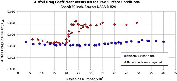
FIGURE 8-63 The effect of surface finish on the minimum drag of an airfoil. The smooth airfoil is only slightly affected by the change in Re, whereas the unpolished camouflage paint job experiences a doubling in magnitude at Re around 20 × 106. (Based on Ref. [23])
The effect of a contaminated leading edge (LE) is also presented in Ref. [23] and is reflected in the drag polar in Figure 8-64. The drag polar, initially smooth, is shifted sharply upward as a consequence of grain contamination as small as 0.004 inches. The polar is shifted farther upward when the grain size grows to 0.011 inches; however, even though this is an increase by a factor of three, the drag polar only shifts up by a fraction – the damage is already done. Reference [23] also shows that LE roughness reduces section lift-curve slope and maximum lift coefficient.
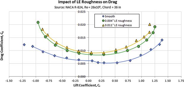
FIGURE 8-64 The effect of introducing surface roughness on the drag polar. (Based on Ref. [23])
8.3.14 Drag Models for Airfoils Using Standard Airfoil Data
Figure 8-65 shows a standard presentation of airfoil drag and pitching moment data from technical documents that all aircraft designers should be intimately familiar with: NACA R-824 [23] and Theory of Wing Sections by Abbott and Doenhoff [44]. The data of interest in this section is the drag polar, which describes the drag coefficient as a function of the lift coefficient. For standard aircraft drag analysis the airfoil is of course only a part of the total aircraft drag; the remaining drag comes from the fuselage, engines, and other parts, as well as the interference of these with each other. However, the airfoil drag is relatively manageable, mathematically, provided a number of rules and realizations are adhered to.
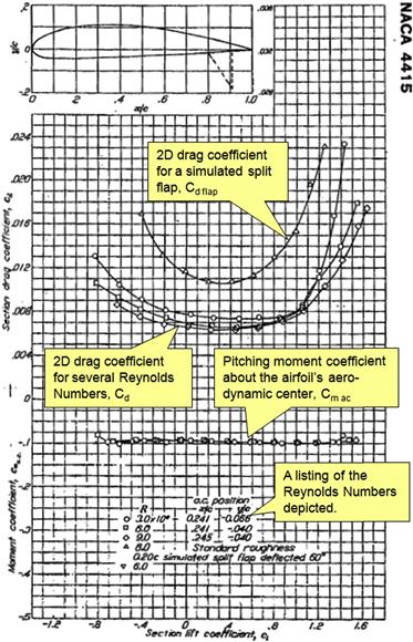
FIGURE 8-65 Typical representation of airfoil data (Ref. [23]).
A considerable amount of information on airfoil drag is at the disposal of the aircraft designer, from the literature, such as the aforementioned NACA publications. Additionally, as stated in Section 8.1.14, Airfoil design, it is even possible to obtain airfoil analysis software, free of charge, from the internet.
8.3.15 Airfoil Selection How-to
The selection of airfoils is often a challenging task for the aircraft designer. The airfoil can have a profound effect on the performance and handling of the aircraft, as well as the structure and weight. If the designer is forced to resort to selecting an airfoil from sources such as the NACA R-824 report or the Stuttgarter Profilkatalog, the following properties should be kept in mind:
Impact on Drag
The geometry of the airfoil will affect where the laminar boundary layer transitions into a turbulent one. This can have a major effect on the magnitude of the skin friction drag and, therefore, the performance of the airplane. The geometry of the airfoil dictates whether or not an airfoil can develop extensive laminar flow. In order to take advantage of NLF airfoils the designer must ensure the mission CL resides inside the drag bucket. If the width of the drag bucket envelopes the CL for best rate of climb, this will also improve climb performance. This can be done by the selection of the appropriate wing area.
Impact on Flow Separation
The geometry also affects at what AOA flow separation begins and how rapidly it grows with additional increase in AOA. Modern NLF airfoils are quite sensitive to imperfections and this may pose a problem if it causes asymmetry between the left and right wings at stall. This may lead to undesirable stall handling, such as an uncontrollable roll-off to the left or right. Additionally, leading edge radius and smoothness for the first 15–20% of the chord can have a significant effect on the stall characteristics.
Impact on Maximum Lift and Stall Handling
The geometry of the airfoil dictates what its maximum lift coefficient will be. The more prominent the camber the higher is the maximum lift coefficient. The smaller the leading edge radius, the lower will be the maximum lift coefficient. A small leading edge radius may also promote a sudden drop in lift at stall, with the associated detrimental effect on stall handling. The shape of the airfoil may also encourage the formation of a separation bubble that may have a profound detrimental effect on stall handling (e.g. see discussion of the NACA 23012 series airfoils in Section 8.2.10, Famous airfoils).
Impact on Longitudinal Trim
The geometry of the airfoil dictates its pitching moment coefficient, Cm. This may have important implications for the sizing of the horizontal tail and trim drag in cruise. Generally, the larger the camber the greater is the magnitude of the pitching moment coefficient. A symmetrical airfoil will have a zero Cm about its aerodynamic center. Cambered airfoils will have negative Cm. Deploying flaps will make it even more negative (stable), but requires a larger horizontal tail area or greater elevator deflection to balance.
Critical Mach Number
The geometry of the airfoil is instrumental in how early the shockwaves begin to form at high subsonic Mach numbers. A thick airfoil will cause a greater local acceleration of air, which will form a shockwave at a lower M than will a less thick airfoil. An airplane designed to cruise at, say, M = 0.5 should not feature airfoils much thicker than 15% without modifying the thickness distribution to prevent shocks at dive speed. This is particularly important in the juncture between the fuselage and wing, where the local airspeeds are even greater.
Impact on Wing-fuselage Juncture
The wing-fuselage juncture can present particularly challenging effects on airflow, where it accelerates to even greater airspeeds than elsewhere on the wing. The effect is generally twofold: acceleration to a higher airspeed means a lower critical Mach number; and acceleration to a higher airspeed means that air must decelerate that much more. If this deceleration (called pressure recovery) takes place over a short distance a flow separation will occur. Such a separation may even take place at a low AOA. The consequence is higher drag and impaired performance.
Impact on Structural Depth
The geometry of the airfoil dictates entirely the structural depth of the wing. A thick airfoil provides a large structural depth that accommodates a taller spar. A taller spar, in turn, brings down bending stresses in the spar caps and results in a lighter wing structure that offers greater fuel volume. For this reason, selecting a thick rather than thin airfoil is essential, as long as it does not increase section drag too much. Modern NLF airfoils are thicker and generate less drag than previous airfoils, which is one of the reasons why established manufacturers design mission-based airfoils.
Evaluation of a Target Zero-lift AOA
It is of importance to identify what zero lift AOA, αZL, to aim for in the airfoil selection process. Using the data of Ref. 23 (Equation [16]), Ref. 13 presents a helpful expression that can be used to estimate target αZL for the selection process. Assuming the designer knows the design AOA, denoted by αi (in degrees), and the design lift coefficient, denoted by Cli, the zero-lift AOA is given by:
Consider an aircraft intended to cruise so its NACA 6-series airfoil is at an AOA near 1° and its section lift coefficient is 0.40. Using Equation (8-63) we readily find the target αZL should be near −2°. Generally, this method is accurate, although it is recommended that test data is used when possible.
Selection of an Airfoil
Assuming the designer is aware of the above limitations and issues, the following guidelines can be kept in mind when selecting an airfoil.
1. If an NLF airfoil is selected for the airplane, look for one with the widest possible drag bucket to help take advantage of its properties (see Figure 8-66). A wide drag bucket makes it likelier that the section lift coefficients (Cl climb and Cl cruise) generated by the wing (or other lifting surfaces) will lie inside it during climb and cruise, regardless of the combination of weight and CG location. The wing area and planform of the airplane must be properly sized to make this possible, otherwise it the section lift coefficients may simply lie outside the drag bucket (see Figure 8-67).
A large wing area results in small values of cruise Cl but an increased skin friction drag. Even though inside the drag bucket the reduction in drag may be less than the rise due to skin friction. Too small a wing area requires a higher climb and cruise Cl and may cause the airplane to operate outside the drag bucket (see Chapter 9, The anatomy of the wing, for guidance). Clearly, the wing must be sized and shaped such that at cruise (for most applications cruise has priority over climb) the values of Cl cruise place it inside the drag bucket. Note that if the reader cannot specifically generate section lift coefficients Cl as a function of spanwise station, the CL may be used, although the limitations of doing this must be understood. The inaccuracy comes into the picture when considering that the magnitude of a section lift coefficient at a specific wing station may be very different from the actual CL. The difference may be large toward the tip or root and this would cause its drag to be greater than the configuration with a larger wing area. Of course, a larger wing area will lower the stalling speed, which is desirable. A wide drag bucket will also improve rate-of-climb and L/D ratio.
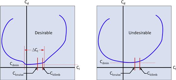
FIGURE 8-66 A drag polar featuring a wide drag bucket (left) is always more desirable than without one (right).
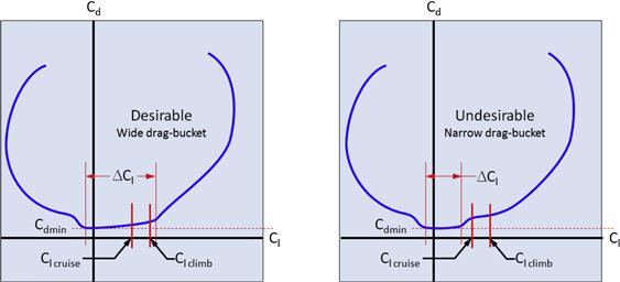
FIGURE 8-67 A drag polar featuring a wide drag bucket (left) is always more desirable than a narrow one (right).
2. Select an airfoil with the largest Clmax possible. However, avoid airfoils with sharp drop in Cl immediately after stall (see Figure 8-68). The sharp drop indicates the presence of a separation bubble near the leading edge on the upper surface of the airfoil, which suddenly combines with the flow separation point near the stall AOA, resulting in a sudden drop in the Cl. This can have very serious consequences for real airplanes. Typically, it causes one wing to stall before the other, resulting in a powerful roll-off that can have profound impact on production flight testing. It is very costly to manufacturers to have to fix the stall characteristics of production airplanes. Always place a great emphasis on good stall characteristics even if it means a loss of a few knots in cruise.
NACA reports often present the ratio Clmax/Cdmin as a figure of merit for designers evaluating airfoils. This implies that the greater the ratio, the farther apart are the two arguments and the better the airfoil. A high Clmax and low Cdmin, what more can one ask for? Well, one can ask for something more – good stall characteristics. The ratio Clmax/Cdmin alone does not tell the whole story. It does not say anything about stall characteristics. Therefore, the ratio should be prefaced with: the greatest ratio Clmax/Cdmin that has benign stall characteristics.
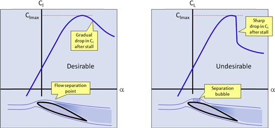
FIGURE 8-68 A sharp drop in Cl at stall (right) is undesirable, as it usually leads to poor stall characteristics.
3. After having identified airfoils with low enough Cdmin and high enough Clmax select the one with the lowest CmC/4 possible at the cruise Cl (see Figure 8-69). However, this coefficient should have less weight in the selection process than the other two. It should be used to pick between two airfoils that happen to offer similar values of Cdmin and Clmax. While the lower Cm C/4 will help reduce trim drag, it can always be accommodated by a proper sizing of the stabilizer.
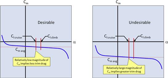
4. Ideally, the maximum L/D ratio (LDmax) should be achieved close to the cruise AOA. Unfortunately, in practice, the two AOAs are separated by a wide margin. Therefore, when considering two airfoils that offer the same LDmax, place a higher weight on the one whose AOA of LDmax is closer to the cruise AOA. A higher LD at cruise yields a more efficient aircraft.
As an example consider the graphs of Figure 8-70. These show a convenient method to check how the applicable lift and drag curves match the intended performance characteristics. The two plots compare the aerodynamic properties of NACA 23015 and 652-415 airfoils. They assume some hypothetical targets for the cruise and climb lift coefficients. For instance, the cruising speed requires the lift coefficient to vary between 0.25 < CLC < 0.32 (depending on weight) and the climb lift coefficient is expected to be close to CL CLIMB ≈ 0.7.
Figure 8-70 also shows that not only does the cruise range reside inside the drag bucket of the NACA 652-415 airfoil, the climb lift coefficient is much closer to the its maximum L/D than that of the NACA 23015 airfoil. An airplane using the NACA 652-415 airfoil will be more efficient than one featuring the 23015 airfoil. It can also be seen that the wing with the NACA 23015 must be installed at a higher angle of incidence than the NACA 652-415 airfoil (these depend on the 3D geometry of the wing).
Additionally, while the NACA 652-415 results in a slightly higher stalling speed, its stall characteristics are far more benign.
To exemplify the selection process, consider the airfoil selection for a new airplane design. To help with the process, Table 8-8 is prepared. It contains three example airfoils whose pertinent properties have been tabulated to allow them to be scored against one another. The data for the candidate airfoils was obtained by digitizing the appropriate graphs in Ref. [23] and, then, after simple analyses, their properties were entered as depicted in the graphs.
While established aircraft manufacturers often design airfoils that are specifically tailored to the mission of the aircraft, the comparison performed in Table 8-8 is still helpful when evaluating custom airfoils.
In this example the airfoils are scored by simply entering a ‘1’ for a winning airfoil in the columns on the right-hand side. The numbers 1, 2, and 3 refer to the three airfoils. Then, the score for each airfoil is summed and the total is entered at the bottom of the table. The airfoil with the highest score is obviously the one to consider, although the results may be more ambiguous than that. Sometimes more than one airfoil simultaneously meets a given criterion – in which case all the appropriate airfoils receive a ‘1’. An example of this can be seen in the table, in lines 8, 15, and 24. Other times, two or more airfoils end up with a total score that is identical. In this case the process must be polished some more. For instance, there could be a weighting factor associated with some of the criteria. For instance, a score of 2 can be given for the lowest drag coefficient, 0.5 for the highest pitching moment coefficient, and so on. The designer can also add other criteria to the table to help with the selection process as well.
While most of the rows in Table 8-8 are self-explanatory, a few need to be elaborated on.
Rows 11 and 12: as a rule of thumb, we expect the three-dimensional lift coefficient to be close to 85–90% of the two-dimensional one. The score here is based on the fact that this places Airfoil 1 inside the cruise range of the CL, but the others outside it.
Row 16: note that Airfoil 1 has the most favorable Cl of Cdmin for cruise. Airfoil 2 (NACA 23015) has it closer; however, it is at a lower value than the cruise CL. For this reason, the airplane would have to be diving to benefit from it. This is further supported by the data in rows 21 and 22, which show that the drag bucket for the 23015 airfoil (if we want to call it that) ranges from Cl = 0 to 0.1, which is beyond where the airplane will be operated. For Airfoils 1 and 3, on the other hand, the cruise Cl is guaranteed to be inside the drag bucket.
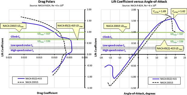
FIGURE 8-70 The aerodynamic characteristics of two airfoils plotted to compare their characteristics to the target performance. Note how well (or poorly) the desired CL for climb and cruise coincide with the airfoil properties. For instance, notice how the LDmax of the NACA 65-series airfoil falls close to the target climb CL (this is very desirable). Also notice how the low- and high-speed cruise CLs are inside the drag bucket for both airfoils, although the 65-series airfoil yields a substantially lower Cd (as long as laminar flow can be achieved) than the five-digit airfoil.

NACA Recommended Criteria
The conclusion section of Ref. [23] lists a number of things to keep in mind when selecting airfoils. These are paraphrased below.
Airfoils permitting extensive laminar flow, such as the NACA 6- and 7- series, have substantially less drag at typical cruise lift coefficients than other kinds of airfoils. However, these characteristics are realized only if the quality of the lifting surface is smooth. Wind tunnel tests have shown that extensive laminar flow is possible on smooth three-dimensional wings if the surface quality is smooth and like that provided by sanding in the chordwise direction with No. 320 carborundum sand paper.
Wings of moderate thickness ratios with such surface qualities can achieve a minimum drag coefficient of the order of 0.0080. In fact, the CDmin depends more on the surface quality than on the chosen airfoil. Thus, at high Reynolds numbers where laminar flow is no longer achievable, drag can be kept low by ensuring smooth surface qualities.
The maximum lift coefficient for moderately cambered 6-series airfoils are as high as those achieved using NACA 24- and 44-series airfoils. The NACA 230-series airfoils with thickness ratio less than 20% generally achieve the highest maximum lift coefficients. The maximum lift coefficient with flaps is about the same for moderately thick 6-series airfoils as it is for the NACA 23012 with flaps. However, the thinner 6-series airfoils have substantially lower Clmax with flaps. The lift curve slope for smooth 6-series airfoils is slightly steeper than that of the 24-, 44-, and 230-series airfoils. It exceeds the theoretical value (2π) for thin airfoils.
Leading edge contamination (roughness) causes large reductions in Clmax for plain and flapped airfoils. The magnitude of the reduction is similar for both. The leading edge contamination also reduces the lift curve slope, especially for thicker airfoils that have the location of minimum pressure farther aft than do thinner ones. This lends support to the importance of understanding the impact of poor surface quality and leading edge contamination on the overall characteristics of the airfoils and, thus, the performance of the aircraft when designing wings.
The NACA 6-series airfoils have higher critical Mach numbers than the earlier airfoil types at typical cruise lift coefficients. However, their critical Mach numbers are lower at higher lift coefficients than are the same types of airfoils. The 6-series airfoils also offer better lift coefficients at higher Mach numbers than the earlier airfoils.
Exercises
(1) The purpose of this exercise is to train the student in retrieving information from the available literature. Here, information from NACA R-824 will be used. It is available for download (free of charge) from the NASA Technical Report Server (http://ntrs.nasa.gov/search.jsp). Perform the following tasks for the NACA 23012 airfoil:
(a) Locate the Station and Ordinate table (p. 359) and plot the airfoil assuming a wing chord of 39.4 inches (100 cm). This task can easily be accomplished using spreadsheet software such as Microsoft Excel. More specifically, plot the upper, lower, and mean-lines. Also determine the x-locations of the airfoil’s maximum thickness and camber.
(b) Using the graph of p. 375, determine the critical Mach number (Mcrit) of the airfoil at a lift coefficient Cl = 0.30.
(c) Using the graph of p. 404, determine the following characteristics for Reynolds numbers of 3 and 6 million. For the Re of 6 million, use both the “clean” and “standard roughness” data. Determine Clmax, Clα of the linear range, “average” Cm for α < 14°, Cdmin, and Cl of Cdmin.
Answers: (b) 0.6, (c) for Re of 3 × 10⁶, Clmax = 1.62, Clα = 0.104, Cm = −0.05, Cdmin = 0.006 and Cl of Cdmin = 0.1.
(2) An airfoil is subjected to airspeed of 315 ft/s on a standard day at S-L, when the pressure at a specific point on it is found to be 13.3 psi. Determine the incompressible and compressible pressure coefficient, Cp, using all three compressibility models of Section 8.3.6, Compressibility modeling.
Answer: −1.702, −1.774, −1.840, and −1.918.
(3) Using the information about the critical Mach number obtained in Exercise (1), determine the critical pressure coefficient, Cp crit, of the NACA 23012 airfoil at the lift coefficient of 0.3.
Answer: −1.294.
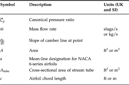

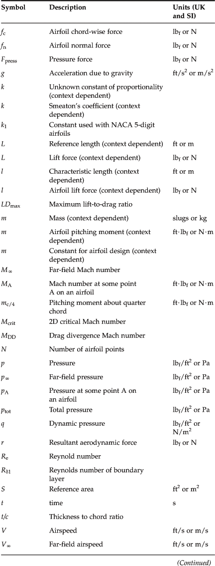
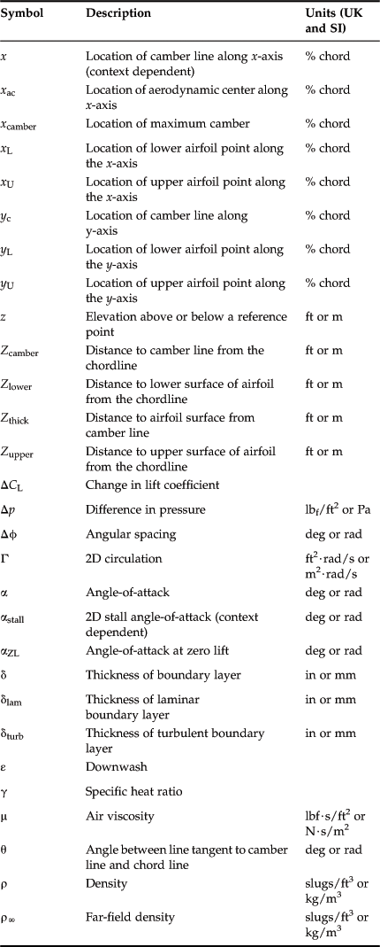
References
1. In: http://wright.nasa.gov/airplane/liftold.html.
2. NACA-TN-2502. Examples of Three Representative Types of Airfoil-Section Stall at Low Speed. McCullough, Goerge B; Gault, Donald E 1951.
3. Smith AMO. High-lift aerodynamics. Journal of Aircraft. 1975;12.
4. Anderson Jr John D. Introduction to Flight. 3rd ed. McGraw-Hill 1989; Section 5.19.
5. Schlichting Hermann. Boundary Layer Theory. Pergamon Press 1955.
6. Young AD. Boundary Layers. AIAA Education Series 1989.
7. Bertin John, J, Smith Michael L. Aerodynamics for Engineers. Prentice-Hall 1979; p. 95.
8. Gopalarathnam Ashok, et al. Design of low Reynolds number airfoils with trips. Journal of Aircraft. 2003;40.
9. Bertin John J. Engineering Fluid Mechanics. Prentice-Hall 1984.
10. Hoak DE. USAF Stability and Control DATCOM. Flight Control Division, Air Force Flight Dynamics Laboratory 1978; Section 4.1.1.3.
11. R.&M. No. 3122 The Formation of Regions of Separated Flow on Wing Surfaces. Aeronautical Research Council, L. F. Crabtree 1959.
12. Kundu, Kumar Ajoy. Aircraft Design. Cambridge University Press 2010.
13. Hoak DE. USAF Stability and Control DATCOM. Flight Control Division, Air Force Flight Dynamics Laboratory 1978; Section 4.1.1.4.
14. In: http://web.mit.edu/drela/Public/web/xfoil/.
15. In: http://www.xflr5.com/xflr5.htm.
16. In: http://www.airfoils.com/index.htm.
17. In: http://aerofoilengineering.com/.
18. Meschia Francesco. Model analysis with XFLR5. Radio Controlled Soaring Digest. 2008;25.
19. NACA TR-460 The Characteristics of 78 Related Airfoil Sections from Tests in the Variable-Density Wind Tunnel. Jacobs, Eastman N, Kenneth E. Ward and Robert M. Pinkerton 1933.
20. NACA TR-492 Tests of 16 Related Airfoils at High Speed. Stack, John, and Albert E. von Doenhoff 1935.
21. NACA TR-537 Tests in the Variable-Density Wind Tunnel of Related Airfoils having the Maximum Camber Unusually Far Forward. Jacobs, Eastman N., and Robert M. Pinkerton 1936.
22. NACA TR-610 Tests of Related Forward-camber Airfoils in the Variable-density Wind Tunnel. Jacobs, Eastman N; Robert M. Pinkerton, and Harry Greenberg 1937.
23. NACA R-824 Summary of Airfoil Data. Abbott, Ira H., Albert E. von Doenhoff and Louis S. Stivers Jr 1945.
24. NASA TM-X-3284 Development of a Computer Program to Obtain Ordinates for NACA 4-Digit, 4-Digit Modified, 5-Digit, and 16 Series Airfoils. Ladson, C. L., and Cuyler W. Brooks Jr 1975.
25. NACA TR-903 Theoretical and Experimental Data for a Number of NACA 6A-Series Airfoil Sections. Loftin, Laurence K., Jr 1948.
26. NASA TM-X-3069 Development of a Computer Program to Obtain Ordinates for NACA-6 and 6A-Series Airfoils. Ladson, C. L., and Cuyler W. Brooks Jr 1974.
27. NASA TM-4741 Computer Program to Obtain Ordinates for NACA Airfoils. Ladson, Charles L., Cuyler W. Brooks Jr., Acquilla S. Hill, and Darrell W. Sproles 1996.
28. NACA TR-947 The Development of Cambered Airfoil Sections having Favorable Lift Characteristics at Supercritical Mach Numbers. Graham, Donald J 1949.
29. NACA R-502 Scale Effect on Clark Y Airfoil Characteristics from NACA Full Scale Wind-Tunnel Tests. Silverstein, Abs, NACA 1934.
30. Riblett Harry. GA Airfoils – A Catalog of Airfoils for General Aviation Use. 5th ed. Self-published 1988.
31. NACA TR-537 Tests in the Variable-Density Wind Tunnel of Related Airfoils having the Maximum Camber Unusually Far Forward. Jacobs, Eastman N., and Robert M. Pinkerton 1936.
32. NASA CR-2443 Development of a Fowler Flap System for a High Performance General Aviation Airfoil. Wentz, W. H., Jr., and H. C. Seetharam 1974.
33. NASA TN D-7428 Low-Speed Aerodynamic Characteristics of a 17-Percent-Thick Airfoil Section Designed for General Aviation Applications. McGhee, Robert J., and William D. Beasley 1973.
34. NACA WR-L-677 Lift and Drag Tests of Three Airfoil Models with Fowler Flaps. submitted by Consolidated Aircraft Corporation Turner, Harold R., Jr 1941.
35. NASA TT-F-749 On Peaky Airfoil Sections. Sato, Junzo 1973.
36. R.&M. No. 3108 Some Effects of Shock-induced Separation of Turbulent Boundary Layers in Transonic Flow past Aerofoils. Aeronautical Research Council, H. H. Pearcey 1955.
37. Pearcey HH. The aerodynamic design of section shapes for swept wings. Advances Aero Sci. 1962;3:277–322 Proceedings of the 2nd International Congress on Aeronautical Science.
38. Whitford Ray. Design for Air Combat. Jane’s 1987.
39. NASA TM-X-1109 An Airfoil Shape for Efficient Flight at Supercritical Mach Numbers. Whitcomb, R. T., and L. R. Clark 1965.
40. Anderson John D. Fundamentals of Aerodynamics. 4th ed. McGraw-Hill 2007.
41. Roskam Jan, Lan Chuan-Tau Edward. Airplane Aerodynamics & Performance. DARcorporation 2000.
42. Glauert H. The effect of compressibility on the lift of an aerofoil. Proceedings of the Royal Society, London, CXVIII 1928; 113–119.
43. Perkins Courtland D, Hage Robert E. Airplane Performance, Stability, and Control. John Wiley & Sons 1949; 59–63.
44. Abbott Ira H, Von Doenhoff Albert E. Theory of Wing Sections. Dover 1959.
45. NACA TN-695 The Effects of Some Surface Irregularities on Wing Drag. Hood, Manley J 1939.
46. Thwaites Bryan. Incompressible Aerodynamics. Dover 1960.
47. NACA WR L-143 Completed Tabulation in the United States Of Tests of 24 Airfoils at High Mach Numbers. Ferri, Antonio 1945.
1This is often spelled Zhukovsky.
2A transition ramp is used to describe the shape of the pressure coefficient curve aft of where it peaks. The ramp can be tailored to modify the adverse pressure gradient to control the transition of the laminar into the turbulent boundary layer without promoting the formation of a large separation bubble.
3This means documents such as Jane’s All the World’s Aircraft, technical data sheets for aircraft, aerospace engineering books, scientific publications, etc.
4An adverse pressure gradient is the rate of rise in pressure from the low pressure peak on the airfoil to the atmospheric pressure aft of the trailing edge. If this pressure rise occurs too rapidly, air will separate and a thick wake will form.