
9.5.2 The Lift Coefficient
The lift coefficient relates the AOA to the lift force. If the lift force is known at a specific airspeed the lift coefficient is obtained from Equation (9-47) and can be calculated from:
![]() (9-50)
(9-50)
In the linear region of the lift curve, at low AOA, the lift coefficient can be written as a function of AOA as shown below:
![]() (9-51)
(9-51)
Equation (9-51) allows the AOA corresponding to a specific lift coefficient to be determined provided the lift curve slope known:
![]() (9-52)
(9-52)
The Relationship between Airspeed, Lift Coefficient, and Angle-of-attack
Consider Figure 9-48, which shows an airplane being operated in horizontal flight at different airspeeds, denoted by the ratio V/VS, where VS is its stalling speed. Starting with the upper left image, the aircraft is at a high airspeed (e.g. if VS = 50 KCAS, the figure shows it at V = 3 × 50 = 150 KCAS). This results in a very low lift coefficient, CL, and an attitude that is slightly nose-down. As the aircraft slows down, it can only maintain altitude by exchanging less airspeed for a higher CL, which calls for a higher α. As it slows down further, a higher and higher nose-up attitude is required to generate a larger and larger CL. Eventually, a maximum value of the CL is achieved, CLmax, after which the airplane can no longer maintain horizontal flight. This is followed by an immediate and forceful drop of the nose caused by the sudden loss of lift. The airplane begins a dive toward the ground, which increases its airspeed, making stall recovery possible. This is shown as the left bottom image, which shows the aircraft recovering and, while in a nose-down attitude, its higher airspeed has already lowered the α.
Wide-range Lift Curve
A typical change in the lift coefficient with AOA ranging from 0° to 90° is shown in Figure 9-49. The graph is based on true wind tunnel test data, although the actual values have been normalized to the maximum lift coefficient. Two important observations can be made. The first is the linear range at low AOA (here shown ranging from AOA = 0° through 10°). Note that the extent of this linear region depends on the geometry and operational airspeeds (via Reynolds numbers). The second observation is the relatively large value of the CL at an AOA around 45°–50°, which, while large, is inefficient because of the high drag associated with it.

9.5.3 Determination of Lift Curve Slope, CLα, for a 3D Lifting Surface
Consider the lift curve slope of an airfoil used for some specific lifting surface (which could be a wing, an HT, or a VT). For reasons that become clear in Section 9.7, Numerical analysis of the wing, the surface induces larger upwash in the flow field than the airfoil alone. Consequently, its effective AOA is less than that of the airfoil (because the induced AOA is larger). Therefore, the wing must operate at a larger AOA to generate the same lift coefficient as the airfoil. The lift curve slope for the wing is less steep than for the airfoil. This fact is used to derive the following expressions that allow the two-dimensional lift curve slope of an airfoil (Clα) to be converted to three-dimensions for a wing (CLα).
The transformation is usually derived using Prandtl’s Lifting Line Theory (see Section 9.7.2, Prandtl’s lifting line method – special case: the elliptical wing). The following expression is used with elliptical wings only:
Lift curve slope for an elliptical wing:
![]() (9-53)
(9-53)
A common (but not necessarily correct) assumption is that the lift curve slope of an airfoil is 2π. This yields the following expression:
Elliptical wing with Clα = 2π:
![]() (9-54)
(9-54)
NACA TN-817 [20] and TN-1175 [21] present methods to make Equation (9-54) suited for AR < 4, but these are generally unwieldy. The following expression is an attempt to extend Equation (9-53) to more arbitrary wing shapes and requires the correction factor, τ, to be determined:
Lift curve slope for an arbitrary wing:
![]() (9-55)
(9-55)
The factor τ is a function of the Fourier coefficients determined using the lifting line method and represents the following correction to the induced AOA, as shown in Dommasch [22]. The actual value of τ is calculated and provided by Glauert [23].
![]()
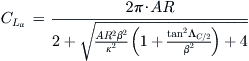
By making some approximations and determining the downwash at the ¾ chord station, rather than the ¼ station, Helmbold [24] derived the expression shown below:
Finally, the following expression, referred to as the Polhamus equation, is derived from NACA TR-3911 [25] and is based on a modification made to Helmbold’s equation. It is also presented in USAF DATCOM [26]. The expression accounts for compressibility, deviation from the 2π airfoil lift curve slope, and taper ratio. While TR does not explicitly appear in the equation, Reference [25] demonstrates that if the mid-chord sweep angle (ΛC/2) is used, the TR can be eliminated. The resulting expression is only valid for non-curved planform shapes and M ≤ 0.8:
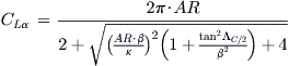 (9-57)
where
β = Mach number parameter (Prandtl-Glauert) = (1 − M2)0.5
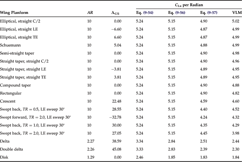
Of the above methods, Equation (9-57) compares well with experiment (and this author’s experience). This can be assessed indirectly by comparing results using it to that of the vortex-lattice method (VLM), which, as has been shown before, compares well with experiment. Such a comparison is shown in Table 9-7. The general trend is that Equations (9-54) and (9-56) (intended for elliptical planform shapes) predict steeper lift curve slopes than Equation (9-57) and the VLM. Also, note the insensitivity of Equations (9-54) and (9-51) to other characteristics, such as sweep and general planform shape of of the wing.
Derivation of Equation (9-53)
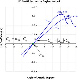
The graph in Figure 9-50 shows the lift curve for two ARs; AR = ∞ (an airfoil) and an elliptical wing of an arbitrary AR. The lift coefficient for the airfoil can be written as follows:
![]()
The wing induces upwash that reduces the α by an amount denoted by αi (induced AOA). Therefore, the lift coefficient for the wing is given by:
![]()
The value of αi is given by Equation (9-87). Inserting this yields:
![]()
The lift curve slope can now be found by differentiating with respect to α:
![]()
QED

9.5.4 The Lift Curve Slope of a Complete Aircraft
A complete aircraft typically consists of a wing, a stabilizing surface, such as a horizontal tail or a canard (or both), a fuselage, and, sometimes, engine nacelles and external stores. All of these components contribute to the total lift developed by the aircraft and, often, their contribution causes the lift curve slope of the aircraft to differ from that of the wing alone. It can be seen that, for instance, the HT produces lift that adds to the wing lift (assuming a fixed neutral elevator). If the combination is attributed to the reference wing area alone, it would “appear” the wing is generating greater lift than its actual contribution. This is important to keep in mind when considering gust loads for airframe loads and in some stability and control analyses. The following method can be used to estimate the total lift curve slope of a wing and HT, approximating that of the complete aircraft. Effectively, we want to write the total lift coefficient of the airplane, ![]() , as follows:
, as follows:
![]() (9-58)
(9-58)
where the zero AOA lift and lift curve slope are computed from:
![]() (9-59)
(9-59)
![]() (9-60)
(9-60)
where
Derivation of Equations (9-59) and (9-60)
We can write the total lift of the wing and HT as follows:
![]()
Divide through by qS to get the lift coefficient form:
![]()
Expand in terms of component properties:
![]()
Insert the AOA the HT is subjected to:
![]()
And finally, gather like terms to yield Equations (9-59) and (9-60):
![]()
QED
9.5.5 Step-by-step: Transforming the Lift Curve from 2D to 3D
An important part of working with airfoils is the realization that the lift capabilities of a two-dimensional airfoil are superior to that of a three-dimensional wing. Figure 9-11 reveals how a two-dimensional lift curve changes once it is introduced to a wing of finite aspect ratio. Among noticeable effects is a reduction in the lift curve slope and lift at zero AOA. The maximum lift coefficient is reduced although the stall AOA increases. This section presents a method that allows the t tnq ransformation of the two-dimensional lift curve into a three-dimensional one. The method assumes the same airfoil along the wing. If more than one airfoil is used, the properties of the airfoil at the MGC can be assumed.
Step 1: Compute a three-dimensionl lift curve slope using Equation (9-57).
Step 2: Compute the zero-lift angle for the two-dimensional airfoil using the following expression, which is obtained by inspection of the curves in Figure 9-51:
![]()
Step 3: Compute lift at AOA = 0° for the three-dimensional wing using:
Step 4: Compute pitching moment for three-dimensional wing, denoted by ![]() . Note that since:
. Note that since:
![]()
![]() (9-62)
(9-62)
EXAMPLE 9-8
A Hershey-bar wing (λ = 1) with an aspect ratio of 20 is being evaluated for use in a low-speed vehicle (M ≈ 0). One of the airfoils being considered is a NACA 23012. Convert the following two-dimensional data for the airfoil (which has been extracted from the Theory of Wing Sections, by Abbott and Doenhoff) for the three-dimensional:
The last expression is obtained from interpolation.
Solution
Step 1: Compute a 3D lift curve slope using Equation (9-57):

where
β = Mach number parameter (Prandtl-Glauert) = (1 − M2)0.5 ≈ 1
κ = ratio of 2D lift curve slope to 2π = 0.1051 × (180/ π)/(2π) = 0.95840
Λc/2 = sweepback of mid-chord = 0°
![]()
Step 2: Compute zero lift angle for the two-dimensional airfoil:
![]()
Step 3: Compute lift at zero angle for the 3D wing using:
![]()
Step 4: Compute pitching moment for three-dimensional wing:
![]()
9.5.6 The Law of Effectiveness
Consider the estimation of the three-dimensional lift curve slope of a wing that has two distinct airfoils at the root and tip. As we have seen, the estimation of the wing’s lift curve slope requires a representative two-dimensional lift curve slope of an airfoil, but which should be used? The law of effectiveness is a handy rule of thumb that helps solve this problem. This law contends that any representative two-dimensional aerodynamic property of a multi-airfoil wing can be approximated by the value at its area centroid, or the mean geometric chord (MGC). A mathematical representation is given by the following equation, obtained using a linear parametric equation:
![]() (9-63)
(9-63)
where P stands for property. The property can be the lift curve slope, maximum lift coefficient, drag coefficient, pitching moment, and similar. When applied to a wing for which we intend to determine a representative lift curve slope, Equation (9-63) becomes:
![]() (9-64)
(9-64)
9.5.7 Flexible Wings
The high-aspect-ratio wings of sailplanes tend to flex excessively during maneuvers and even in normal flight. Flex as large as 6 ft (2 m) is not unheard of in some cases. The same phenomenon occurs on many commercial aircraft (e.g. Boeing 747 and Airbus A380). Regardless of aircraft class, if excessive wing flex is anticipated, it is important to consider its effects on the lift capability of such aircraft.
Figure 9-52 shows the effect of wing flex on the distribution of section lift coefficients. In this example, a wing with a 50-ft wingspan is deflected so its tip is 5 ft higher than that of the unflexed wing. The figure shows that for a given AOA, the center of lift moves inboard, reducing the bending moment. However, less lift is also being
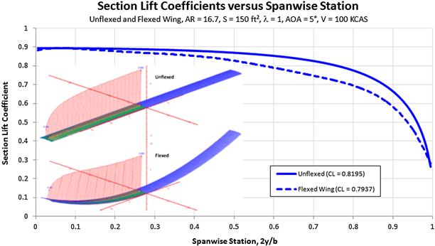
produced (in this particular case, some 3% less), so the resulting aircraft will have to operate at a higher AOA. This will lead to a slightly higher operational lift-induced drag and will diminish the wing’s long-range efficiency. Additionally, the lift curve slope reduces by about 3%. While this may sound detrimental, there are actually two sides to the topic; the other is discussed in Section 10.5.9, The polyhedral wing(tip).
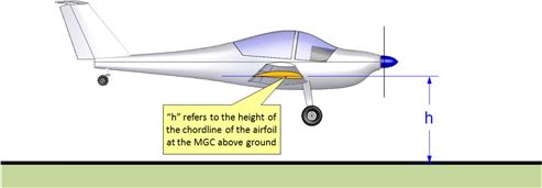
9.5.8 Ground Effect
Ground effect is the change in the aerodynamic forces as a consequence of the body being in close proximity to the ground. As the aircraft nears the ground, the ground will get in the way of the downwash, effectively preventing it from fully developing. This modifies the entire flow field around the aircraft and, thus, affects a number of its characteristics. Some formulation indicates the aerodynamic properties of the airplane begin to change when it is as much as 2 wingspans from the ground. However, the changes are negligible at that height and it is more reasonable to include ground effect once the airplane is about 1 wingspan from the ground or less. Pilots begin to detect those effects at an even lower height, typically around half a wingspan.
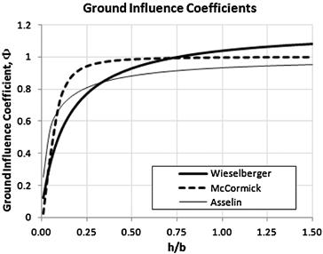
The problem of ground effect was studied as early as 1912 by Albert Betz [27] (1885–1968). Using Prandtl’s lifting line theory, Wieselberger [28] developed a formulation to estimate the reduction in the lift-induced drag near the ground. His work is translated in Ref. [29]. It does this by calculating a special ground influence coefficient, denoted by Φ. The presentation here resembles that of Ref. [30], in which h stands for height of the wing above the ground and b is the wingspan. It differs only slightly from the presentation of Wieselberger, who used h/2 for the height above the ground. Additionally, in order to correspond to the other two presentations shown below, Wieselberger's coefficient (denoted by σ) is subtracted from 1, yielding:
![]() (9-65)
(9-65)
This approximation appears in good agreement with experiment [29] for values of h/b between 0.033 and 0.25. Using the Biot-Savart law applied to a horseshoe vortex whose span is πb/4, McCormick [31] shows that the ground influence coefficient can be estimated from:
![]() (9-66)
(9-66)
Assuming an elliptical lift distribution of a straight wing of AR ≈ 5 and using the lifting line theory, Asselin [32] estimates the following value of the ground influence coefficient:
![]() (9-67)
(9-67)
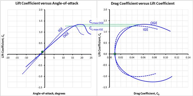
These approximations are compared in Figure 9-54. The ground influence coefficient is then used to adjust the following characteristics of the airplane:
![]() (9-68)
(9-68)
![]() (9-69)
(9-69)
where IGE stands for in ground effect and OGE stands for out of ground effect.
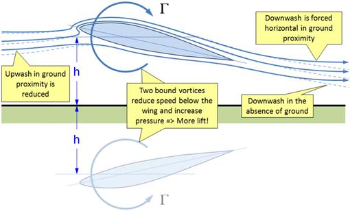
Modeling the ground effect can be accomplished using vortex theories such as Prandtl’s lifting line theory or Weissinger’s vortex-lattice theory. By creating an inverted mirror image of the wing (or airfoil) with bound vortices of equal strength but rotating in opposite directions (see Figure 9-55) the resulting flow field will feature a horizontal streamline along the ground plane. The streamlines above and below will be realigned when compared to the flow field in the absence of the ground as is shown in Figure 9-55. The impact on the lift curve, drag polar, and pitching moment curve is shown in Figure 9-56 and Figure 9-57. The following changes can be noted (these are in part based on Ref. 31). Note that IGE stands for in ground effect and OGE stands for out of ground effect.
(1) Up- and downwash in the proximity of the ground is reduced compared to that in the far-field.
(2) This reduction lowers the induced AOA, resulting in less aft tilting of the lift vector and, thus, less induced drag (see Section 15.3.4, The lift-induced drag coefficient: CDi). The minimum drag, however, is not reduced.
(3) The reduced up- and downwash also reduces the lift. However, the two bound vortices (on either side of the ground plane) will cause a greater reduction in airspeed under the airfoil, increasing the pressure along the lower surface above that in the absence of the ground. This increase is greater than the reduction due to the diminished downwash, yielding an overall increase in lift at a given AOA.
(4) The lift increase causes an increase in the lift curve slope. Based on Ref. [29] this tends to result in a small reduction in the zero-AOA lift.
(5) The steepening of the lift curve slope increases the pitching moment of the wing and shifts it downward.
(6) The effective AR is increased because of the reduction in lift-induced drag. This, and the accompanying increase in lift at a given AOA, increases the L/D ratio, causing a “floating” tendency.
(7) The trim AOA is reduced, which means that the airplane has a tendency to go to a lower AOA.
(8) Elevator effectiveness of a conventional tail-aft configuration is reduced as the low-pressure region on the lower surface is counteracted by the formation of a high-pressure region similar to that of the wing. By the same token, the elevator effectiveness of a canard configuration will increase.

9.5.9 Impact of CLmax and Wing Loading on Stalling Speed
During the design stage the stalling speed and required wing area must be determined. Figure 9-58 highlights how wing loading (W/S) and maximum lift coefficient (CLmax) affect the stalling speed (here shown in KCAS) by displaying it as a carpet plot. The figure shows the regulatory FAR 23 stall speed limit of 61 KCAS for single-engine aircraft and the 45 KCAS limit set forth in the Light Sport Aircraft (LSA) category. The graph has selected aircraft superimposed. Note that single-engine aircraft, such as the PC-12 and TBM-850, are turboprop aircraft that were granted exemption from the 61 KCAS rule on the grounds of envelope protection equipment they feature.
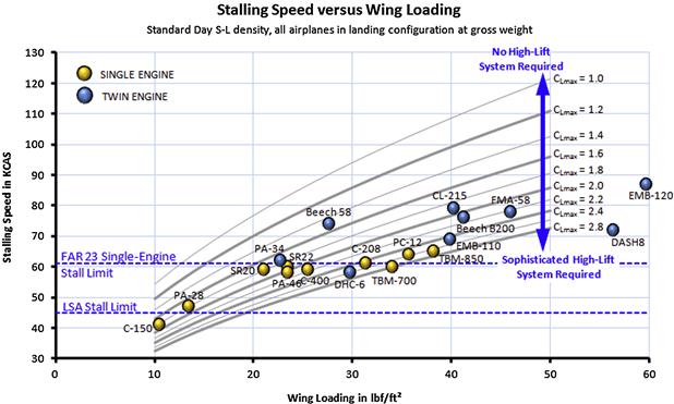
FIGURE 9-58 A carpet plot showing stalling speed as a function of wing loading and maximum lift coefficient.
As an example of use, consider an airplane slated for FAR 23 certification characterized by a wing loading of some 25 lbf/ft2. It can be seen it must feature a high-lift system capable of at least CLmax = 2.0 in order to meet the 61 KCAS requirement.
Alternatively, consider another example in which the designer of an airplane slated for FAR 23 certification wants to feature a simple high-lift system capable of CLmax = 1.8. Figure 9-58 reveals that as long as the wing loading is less than 22 lbf/ft2 the FAR 23 single-engine stall speed limit (61 KCAS) will be complied with. The following expression is used to plot the curves in Figure 9-58, of which the right hand approximation is only valid at S-L. The constants (1/1.688 = 0.592 and 29/1.688 = 17.18) convert the value in ft/s to knots.
![]() (9-70)
(9-70)
9.5.10 Step-by-step: Rapid CLmax Estimation [5]
The primary purpose of this method is to allow a fast estimation of a likely stalling speed. This method is very simple and, consequently, accuracy is suspect. It is presented here because it is acknowledged that, during the conceptual design stage, the designer needs a fast and simple method that has a “fair chance” of providing reasonably accurate results. It is acceptable only during the conceptual design phase and should be replaced with more accurate methods, once the design progresses.
Step 1: Calculate a representative Clmax (two-dimensional) for the airfoil at the MGC using the law of effectiveness:
![]() (9-71)
(9-71)
Step 2: Calculate the three-dimensional CLmax from the following expression (this is the straight wing CLmax):
![]() (9-72)
(9-72)
Step 3: Correct for wing sweep angle. This reduces the maximum lift over that of a straight wing, highlighting yet another challenge for the operation of aircraft with swept wings. Generally, the reduction in the maximum lift can be estimated from the following expression:
![]() (9-73)
(9-73)
where
CLmax0 = max lift coefficient of the unswept wing
KΛ = Sweep correction factor (see Figure 9-59)
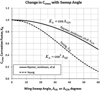
Raymer [5], Jenkinson [33], and others define KΛ as follows, where it is based on the sweep of the quarter-chord:
![]()
Young [34], on the other hand, defines it in terms of the leading edge sweep. It matches historical data well:
![]()
For instance, a wing sweep of 35° will reduce the CLmax by about 15% per Figure 9-59. Note that these methods are also extended to evaluate the reduction in effectiveness of control surfaces with swept hingelines. In this case, replace ΛC/4 by the hingeline sweep angle.
EXAMPLE 9-9
Compare the calculated maximum lift coefficient for the Cirrus SR22 using the Rapid CLmax Method and compare to the “known” value of CLmax of the airplane, which can be calculated using published information in the aircraft’s POH (S = 144.9 ft2, W = 3400 lbf, and VS = 70 KCAS [M = 0.10]) and the calculated values of Table 16-6. Assume the airfoil for the airplane is NACA 652-415 for both the root and tip.
Solution
Start by estimating the maximum three-dimensional lift coefficient to compare to, based on the POH information:
![]()
Next, let’s figure out the Reynolds number at stall, using the average chord for the airplane (in lieu of the MGC). The average chord can be found from Equation (9-17):
![]()
Therefore, using Equation (8-28) the Reynolds number equals:
![]()
We use this information to extract the maximum lift coefficient for the NACA 65-415 airfoil using the wind tunnel data in NACA R-824 [35]. Using the plot for Re = 3.0 million (which is closest to 2.86 million), displayed in Figure 9-60, the Clmax = 1.45 and this will be used at the root.
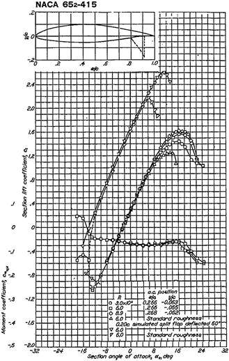
FIGURE 9-60 Lifting properties of the NACA 65-415 airfoils. (from Ref. [34])
Since the airplane’s taper ratio is 0.5, the Re at the root is two times that at the tip. By inspecting the graph in Figure 9-60 it is estimated that the tip Clmax is approximately 1.35. Therefore, the 3D CLmax for the SR22, assuming NACA 65-415 for root and tip, can be estimated as follows:
By observation, the quarter-chord sweep angle is 0°. Therefore, the three-dimensional maximum lift coefficient can be found to equal:
![]()
The difference between the POH and estimated value using the POH is some 10% – in this case, underestimating the capability of the airplane. That level of accuracy could adversely affect the wing sizing of a brand-new aircraft and must be kept in mind, although it will give some idea of the maximum lift coefficient. However, the method does not account for the lift generated by the fuselage and HT at this high AOA.
9.5.11 Step-by-step: CLmax Estimation per USAF DATCOM Method 1
The wing’s maximum lift coefficient can also be calculated using the following method from the USAF DATCOM (where it is referred to as Method 1). This method requires access to an accurate wingspan-wise loading analysis program, such as the vortex-lattice or doublet-lattice methods. The method is limited to moderately swept wing planforms, where LE vortex effects are not yet significant. Delta wings are excluded, unless the LE vortex can be estimated. Furthermore, the spanwise location where stall is first detected should be limited within a band extending from one local chord-length away from the wing root and tip. The DATCOM considers this method superior to Method 2 (see next section).
Step 1: Determine the Two-dimensional Maximum Lift Coefficient
Determine the 2D Clmax along the span for the wing, based on the appropriate Mach number and Reynolds number. Experimental data should always be used if available.
Step 2: Plot the Distribution of Section Lift Coefficients
Plot the Clmax along a normalized spanwise station (2y/b, ranging from 0 to 1), as shown by the dashed line in Figure 9-61.

Step 3: Determine the AOA at which Local Cl Intersects Clmax
Then plot the distribution of section lift coefficients for an AOA until the maximum of a local Cl intersects the airfoil’s Clmax. This is where the stall will first occur. An approximate value of where this occurs can be estimated from (Ref. [1], Article 4.1.3.4, Wing Maximum Lift) (note that λ = taper ratio):
![]() (9-74)
(9-74)
Step 4: Compute CLmax
Calculate the three-dimensional CLmax by integrating along the span:
 (9-75)
where
Cl(η) = section lift coefficient as a function of spanwise station
C(η) = wing chord as a function of spanwise station
η = spanwise station = 2y/b; ranges from 0 to 1 (for b/2)
EXAMPLE 9-10
Predict the maximum lift coefficient for the Cirrus SR22 using the DATCOM method and compare to the “known” value of CLmax3D (= 1.41), calculated in Example 9-9. Assume the airplane has an airfoil in the NACA 652-415 class and account for the effect of Reynolds number on the Clmax at the root and tip.
Solution
The results in Figure 9-61 were obtained using the vortex-lattice solver SURFACES, but similar data should be obtainable from other solvers as well. The model is based on measurements taken from Figure 16-15 and included the wing’s leading edge extensions (or cuffs), the fuselage, and horizontal tail. Note that the program calculates the total lift coefficient, CL (see values in parentheses in the legend) and these represent values that would be returned by Equation (9-75) if the shape of the lift distribution were to be presented as a function of the spanwise station.
The stall limit (blue straight dashed line) indicates the Clmax = 1.45 at the root of the NACA 652-415 airfoil and 1.35 at tip, determined in Example 9-9. This allows the stall AOA and the maximum lift coefficient to be estimated using the DATCOM method as follows:
![]()
The difference between the POH (CLmax = 1.41) and the estimated value (CLmax = 1.468) is some 4.1% and, indeed, shows a very good agreement. This method generally agrees well with experiment and differs by approximately ±6%.
Finally this; it is acknowledged that not all readers have access to codes like the one used in this example and this may present frustration to some. While the author empathizes with such emotions, ultimately, engineers working in industry have access to such codes and this example is intended for them. It is possible to use the method with the lifting line theory presented in Section 9.7, Numerical analysis of the wing.
9.5.12 Step-by-step: CLmax Estimation per USAF DATCOM Method 2
The wing’s maximum lift coefficient can be calculated using the following method from the USAF DATCOM (where it is referred to as Method 2). While somewhat involved, the method allows the estimation of the maximum lift and angle-of-attack for maximum lift at subsonic speeds. The method is empirically derived and is based on experimental data for predicting the subsonic maximum lift and the angle-of-attack for maximum lift of high aspect ratio, untwisted, constant section wings.
Generally, the maximum lift of high-aspect-ratio wings at subsonic speeds is directly related to the maximum lift of the wing section or airfoil. According to the DATCOM, the wing planform shape influences the maximum lift obtainable, although its effect is less important than that of the airfoil’s section characteristics.
Step 1: Determine the Taper Ratio Correction Factor
First determine if the wing in question complies with the DATCOM’s “definition” of a high-aspect-ratio wing. Do this by determining the taper ratio correction factor (TRCF), C1, from Figure 9-62. Alternatively, the TRCF can be approximated using the following empirical expression, based on the curve of Figure 9-62.
![]() (9-76)
(9-76)
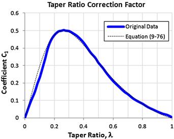
FIGURE 9-62 Taper ratio correction factor. (Based on Ref. [1])
Step 2: Determine if Wing Qualifies as “High AR”
Then determine whether the wing complies with the DATCOM’s “definition” of a high-aspect-ratio wing:
![]() (9-77)
(9-77)
If the airplane’s AR is larger than the ratio of Equation (9-77) then the procedure is applicable to it.
Step 3: Determine the Leading Edge Parameter
Determine the leading edge parameter (LEP), denoted by Δy, which is used several steps later. The parameter Δy is the difference between airfoil ordinate at 6% chord and ordinate at 0.15% chord and is represented in terms of %. Thus, a value of 0.03 would be written as 3.00. Since this method assumes a single airfoil wing, it is appropriate to approximate the leading edge parameter based on the geometry of the airfoil at the mean geometric chord. Figure 9-63 illustrates the process. Note that this is based on an airfoil ordinate table that has been normalized to a chord of unity (C = 1).
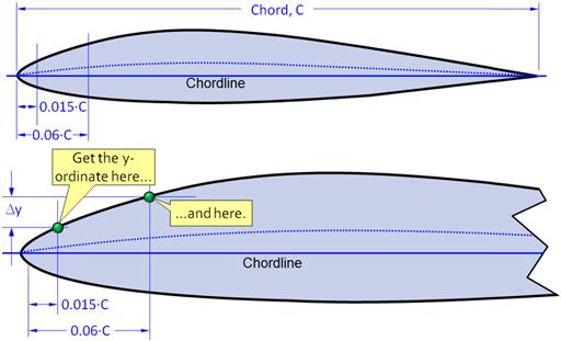
FIGURE 9-63 Determination of the LEP. (Based on Ref. [1])
The listing below contains expressions for the LEP, Δy, for selected types of airfoils, based on their thickness-to-chord ratios (t/c). The explicit expressions in the list may make it easier to determine Δy without having to perform calculations based on the ordinate table. The list is based on Figure 2.2.1-8 of the USAF DATCOM [1].
Step 4: Determine the Max Lift Ratio
Determine the ratio ![]() using Figure 9-64. The figure illustrates the variation of the ratio between the wing’s maximum lift coefficient and the section maximum lift coefficient as a function of the leading edge sweep and the LEP Δy:
using Figure 9-64. The figure illustrates the variation of the ratio between the wing’s maximum lift coefficient and the section maximum lift coefficient as a function of the leading edge sweep and the LEP Δy:
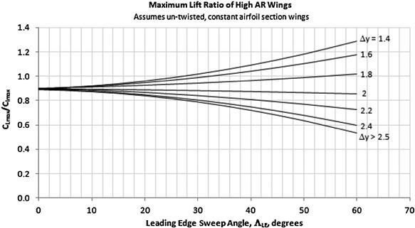
FIGURE 9-64 CLmax/Clmax ratio data plot. (Based on Ref. [1])
where
Step 5: Determine the Mach Number Correction Factor
Determine the Mach number correction factor (MNCF), ΔCLmax, from Figure 9-65, using the LEP, the wing’s leading edge sweep (ΛLE), and Mach number evaluated at the stalling speed. Note that the reference document also presents similar graphs for ΛLE = 40° and 60°, but such sweeps are rarely used on GA aircraft.
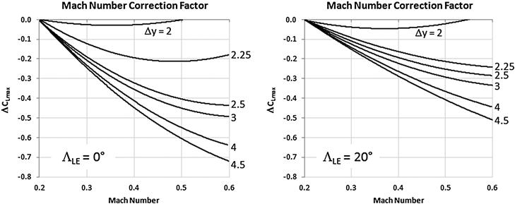
FIGURE 9-65 Determine ΔCLmax using the above graphs. (Based on Ref. [1])
Step 6: Calculate the CLmax
Calculate the wing’s maximum lift coefficient CLmax using the expression below:
![]() (9-85)
(9-85)
where
![]() = ratio obtained from Figure 9-64
= ratio obtained from Figure 9-64
![]() = section maximum lift coefficient
= section maximum lift coefficient
![]() = Mach number correction factor obtained from Figure 9-65
= Mach number correction factor obtained from Figure 9-65
Step 7: Determine Zero Lift Angle and Lift Curve Slope
Determine the wing’s zero lift angle, αZL, and lift curve slope, CLα. Both have to be in terms of degrees.
Step 8: Determine a Correction for the Stall Angle-of-attack
Determine the correction angle, ![]() , for the nonlinear effects of vortex flow from Figure 9-66.
, for the nonlinear effects of vortex flow from Figure 9-66.

FIGURE 9-66 Determine Δαstall using the above graphs. (Based on Ref. [1])
Step 9: Determine the Wing Stall Angle-of-attack
The angle-of-attack of the wing a stall can be calculated from the following equation:
![]() (9-86)
(9-86)
where
EXAMPLE 9-11
Compare the calculated maximum lift coefficient for the Cirrus SR22 using the DATCOM method to the known value of CLmax for the airplane, calculated as shown in Example 9-9.
Solution
All values in this solution were obtained by scaling the airplane in the 3-view (see Figure 16-15) based on the indicated wingspan. A reader trying to reproduce the solution may come up with slightly different dimensions.
Based on the 3-view, the leading edge sweep angle was found to equal: ΛLE = 1.93°
The aspect ratio is found using the wingspan and area information in the 3-view:
![]()
Using Figure 16-15 the taper ratio is estimated to be 0.5. Additionally, the leading edge parameter Δy for the NACA 65-415 airfoil is approximately 2.86%, obtained using Equation (9-81).
The wing was checked to see if it complies with the DATCOM definition of a high AR wing. To do this, we calculate the taper ratio correction factor using Equation (9-76), which turns out to be C1 = 0.3064.
Therefore, from Equation (9-77):
![]()
This simply means that the method is applicable to the SR22. Next read Figure 9-64 to determine the ratio CLmax/Clmax. The resulting ratio is approximately:
![]()
Note that a maximum section lift coefficient is estimated at ![]() , using Figure 9-60 (and as shown in Example 9-9). Next, let’s estimate the Mach number correction factor (MNCF), ΔCLmax. We do this using Figure 9-65 with ΛLE = 0 (since the LE sweep is only 1.93°), M = 0.10 and Δy = 3.5:
, using Figure 9-60 (and as shown in Example 9-9). Next, let’s estimate the Mach number correction factor (MNCF), ΔCLmax. We do this using Figure 9-65 with ΛLE = 0 (since the LE sweep is only 1.93°), M = 0.10 and Δy = 3.5:
![]()
We can now estimate the three-dimensional maximum lift coefficient for the wing using Equation (9-85):
![]()
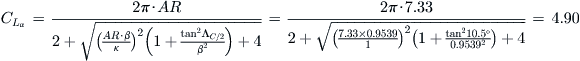
The difference between the POH and estimated value using the POH is some 11.6%. Next, estimate the stall AOA. We do this by first estimating the lift curve slope for the SR22 using Equation (9-57), repeated for convenience.
where
AR = wing aspect ratio = 10.12
β = Mach number parameter (Prandtl-Glauert) = (1 − M2)0.5 ≈ 0.995. Call it 1
κ = ratio of 2D lift curve slope to 2π = 0.107 × (180/π)/(2π) = 0.9757
Λc/2 = sweepback of mid-chord is close 0°
![]()
From Table 8-5, the zero-lift angle for the 652-415 airfoil is αZL = −2.6°. Next, let’s determine the nonlinear vortex flow-correction angle from Figure 9-66. Using the leading edge sweep angle ΛLE = 1.93° and the leading edge parameter Δy = 2.86%, the correction angle is approximately ![]() . This allows us to calculate the stall angle-of-attack using Equation (9-16):
. This allows us to calculate the stall angle-of-attack using Equation (9-16):
![]()
The actual stall angle for the SR22 is not published, so a comparison cannot take place. However, it is thought that this angle is probably 1° to 3° too low.
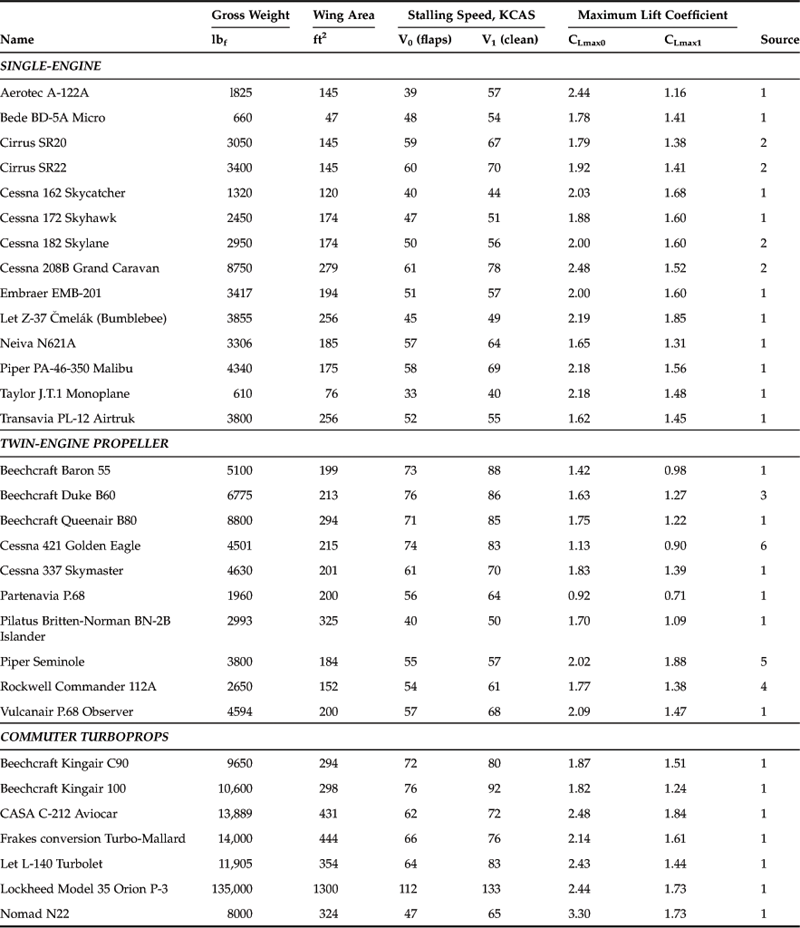
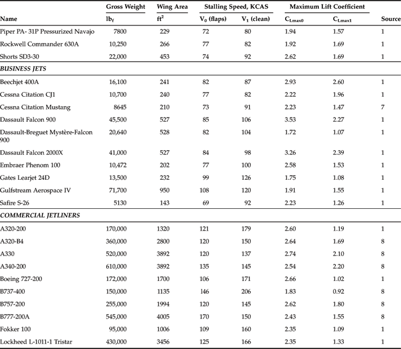
9.5.13 CLmax for Selected Aircraft
Examples of the maximum lift coefficient for selected aircraft are shown in Table 9-8. The aspiring designer is encouraged to be realistic and careful when estimating this value. It has a profound impact on the capability of the aircraft; an overestimation inevitably results in an undersized wing area, which could have a major impact on the stall and low speed characteristics of the new design. Always compare your maximum lift coefficient to that of similar aircraft to ensure unrealistic overestimation is avoided.
TABLE 9-8
Maximum Lift Coefficients for Selected Aircraft
Sources:
1. Jane's All the World's Aircraft
3. http://www.classg.com/aircraft_specs.i?cmd=compare&manid1=56&model1=60+Duke
4. http://www.classg.com/aircraft_specs.i?cmd=compare&acids=568%2C520%2C172%2C922&replaceid=520&manid2=89&model2=phenom+100
5. http://www.classg.com/aircraft_specs.i?cmd=compare&acids=568%2C520%2C172%2C922&replaceid=520&manid2=89&model2=phenom+100
6. http://www.aeroresourcesinc.com/store_/images/classifieds/119-1.pdf
9.5.14 Estimation of Oswald’s Span Efficiency
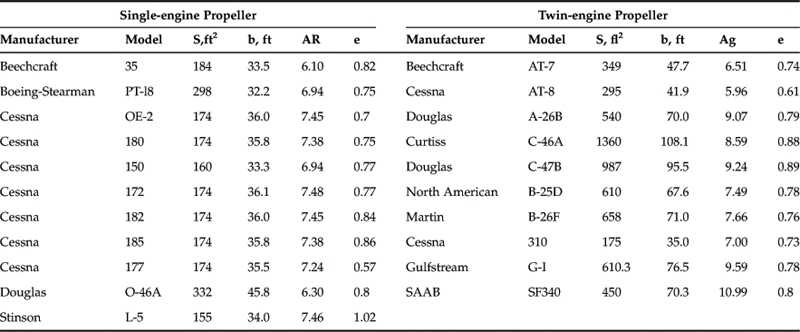
The Oswald span efficiency is a vital parameter required to predict the lift-induced drag of an airplane. It is named after W. Bailey Oswald, who first defined it in a NACA report published in 1933 [36]. Interestingly, Oswald called it the airplane efficiency factor. It is not always easy to estimate, but here several methods will be demonstrated. Note that examples of the Oswald efficiency for selected single- and twin-engine aircraft are shown in Table 9-9.
Basic Definition
The span efficiency can be defined as the resultant of the lift and side force, divided by the product of π, AR, and the lift-induced drag coefficient, as shown below. The expression assumes that CDi is already known, for instance through flight or wind tunnel testing.
If the wing has winglets the aspect ratio should be corrected by modifying the AR using the following expression [32]:
![]() (9-88)
(9-88)
where
Method 1: Empirical Estimation for Straight Wings
Raymer [5] presents the following statistical expression to estimate the Oswald efficiency of straight wings. Note that it omits dependency on taper ratio, but is still handy for conceptual design work. The expression is limited to lower AR only:
![]() (9-89)
(9-89)
Method 2: Empirical Estimation for Swept Wings
Raymer [5] also presents the following statistical expression to estimate the Oswald efficiency of swept wings. It has limitations similar to Equation (9-89):
![]() (9-90)
(9-90)
Brandt et al. [4] present the following expression to estimate the factor:
![]() (9-91)
(9-91)
where
Method 3: Douglas Method
Shevell [37] presents the following expression to calculate the Oswald efficiency, which is in part based on unpublished studies by the Douglas aircraft company. Its presentation has been modified slightly to better fit the discussion here. Other than that, it returns exactly the same values.
![]() (9-92)
(9-92)
where
Method 4: Lifting Line Theory
The lifting line theory is presented in Section 9.7, Numerical analysis of the wing and Section 15.3.4, The lift-induced drag coefficient: CDi. The Oswald span efficiency can be calculated using the method shown in Section 9.7.5, Computer code: Prandtl’s lifting line method.
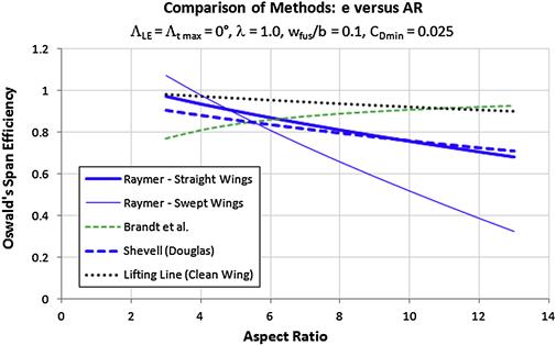
Note that Methods 1 through 4 are compared in Figure 9-67 with a straight Hershey-bar wing. The results for the lifting line theory are theoretical results for a clean wing. Also note that Methods 1 and 2 do not reflect dependency on the taper ratio, λ.
Method 5: USAF DATCOM Method for Swept Wings – Step-by-step
The USAF DATCOM [1, p. 2.2.1-8] is based on a paper by Frost and Rutherford [38] published in 1963. The paper suggests that the Oswald efficiency depends on the factor R, which is the ratio between the actual drag force of a wing and that of an elliptical wing. The idea assumes that both utilize a symmetrical airfoil. Using statistical analysis of a large number of NACA reports, the authors devised a method to estimate the span efficiency for a larger range of AR. Per Ref. [37] the method compared to test data that included following planform and flight conditions:
This does not mean it is not applicable to other planform shapes. The method is used to estimate a special factor, called the leading edge suction parameter, R, which is used with the following expression to estimate the span efficiency:
![]() (9-93)
(9-93)
where R = leading edge suction parameter (must be read from Figure 4.7 in the reference document).
This method requires several parameters to be determined, which are then used to extract the LE suction parameter, R, for use with Equation (9-93).
Step 1: Calculate the Lift Curve Slope
Lift curve slope can be calculated from Equation (9-57) (where the variables are explained):
Step 2: Calculate the Leading Edge Suction Parameter
Leading edge suction parameter:
![]()
where
lLER = leading edge radius (from airfoil data)
μ = air viscosity, in lbf·s/ft2
ρ = air density, slugs/ft3
Step 5: Read or Calculate the Leading Edge Suction Parameter
If ![]() determine R from Figure 9-68 or calculate from the following expression:
determine R from Figure 9-68 or calculate from the following expression:
![]()
If ![]() determine R from Figure 9-68 or calculate from the following expression:
determine R from Figure 9-68 or calculate from the following expression:
![]()
Neither equation is based on theoretical analysis, but rather derived using a curve fit methodology that results in acceptable fit to the graphs.
EXAMPLE 9-12
Determine the Oswald’s span efficiency for the Learjet 45XR, whose AR = 7.33 and TR = 0.391. Compare methods 2 and 4. Assume the airfoil has a section lift curve slope of 2π, a LE sweep of 17°, mid-chord sweep of 10.5°, and a LE radius of 0.1 ft. Assume the maximum thickness is at the mid-chord as well. Assume an airspeed of M = 0.3 at S-L on a standard day (V = 335 ft/s) and ignore the fact the airplane has winglets.
Solution
Method 4
Clearly, there is a range of values to consider, begging the question: which one should we pick? Unless there is confidence in a particular method, this author would take the average of the three (0.812) until a better number is determined.

FIGURE 9-68 Leading edge suction parameter. (Based on Ref. [4])
9.6 Wing Stall Characteristics
All normal airplanes need to exceed a certain minimum airspeed before they can become airborne and maintain level flight. The minimum airspeed required for level flight is the stalling speed. What transpires at this speed arguably inflicts one of the most important design challenges for the wing design, or for that matter, the entire airplane. This section is dedicated to the stall and intended to provide important information about this well-known phenomenon.
It is helpful to visualize the stall maneuver in terms of altitude as well as airspeed. A pilot-controlled stall maneuver is depicted in Figure 9-69. It begins with engine power being cut and a subsequent deceleration. For compliance with 14 CFR Part 23.201, Wings level stall, this deceleration should be as close to 1 KCAS per second as possible.
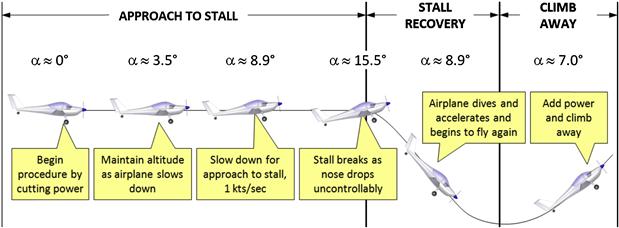
As the airplane slows down, a larger and larger α is required to maintain altitude and the approach to stall phase culminates in the stall itself, as the airplane reachesαSTALL or αCLmax and breaks the stall by the sudden drop of the nose. The drop leads to a dive, which, in turn, results in altitude being lost, as shown in the figure. This altitude loss depends on the size of the aircraft and can be as small as 25–50 ft for a small and light homebuilt or ultralight aircraft; 200–400 ft for a two- to four-seat single-engine GA aircraft; to 2000 ft or more for a large commercial jetliner aircraft. The stall recovery phase ends with power being added and a subsequent climb to altitude.
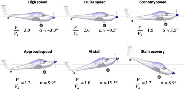
9.6.1 Growth of Flow Separation on an Aircraft
Flow separation can be a serious issue for aircraft and one that the designer must be fully aware of in order to minimize it. Consider the series of images in Figure 9-70, which shows an airplane seen from the same perspective at different airspeeds. Note that the airspeed ratios and AOA are approximate and correspond to the design in the figure only, although they would be applicable to many aircraft types. If the aircraft is well designed there should not be any flow separation regions at the cruising speed. This ensures it will be as efficient as possible at cruise because the flow separation is a source of increased pressure drag. Once slowing down from cruising speed the AOA begins to rise and it is inevitable that separation regions begin to form and increase as well.

FIGURE 9-70 Growth of flow separation region on an aircraft as seen from a fixed point from the aircraft.
As soon as the airplane has decelerated to approximately its economy cruising speed (or best rate-of-climb airspeed), a separation region has already begun to form in two places: mid-span and at the wing/fuselage juncture. This is highly undesirable, but unavoidable. The separation on the wing depends solely on its geometry. For instance, the aircraft shown in Figure 9-70 has a tapered wing planform whose section lift coefficients are highest around the mid span (see Section 9.4.5, Straight tapered planforms), although an attempt has been made here to suppress them at the tip with a geometric wing washout. This causes the flow to begin to separate mid-span rather than elsewhere on the wing. Of course, we seek a progression of the separation that begins at the root and moves toward the tip, but achieving this would require a large wing washout that would be detrimental to the wing’s efficiency, which, by the way, is the reason why a tapered planform was chosen in the first place.
With respect to the flow separation at the wing/fuselage juncture, we must distinguish between separation caused by the high AOA on the wing, and that caused by poor geometry between the two. The former is unavoidable with an increase in AOA, whereas the latter forms prematurely at relatively low AOA, sometimes even before any separation is visible on the wing itself. It is the responsibility of the aerodynamicist to suppress this formation as long as possible and this can be achieved by a careful tailoring of the wing root fairing. The shape of this separation is best described as one having a distinct volume that extends as far as a chord length or more into the flow field behind the juncture. For this reason it is appropriately called a separation bubble. The airplane in Figure 9-70 does not have a wing root fairing in this area, but the formation of the separation bubble should encourage the aspiring aircraft designer to design a fairing to suppress it. The pressure inside it is less than in the surrounding area and, therefore, it increases the drag of the aircraft. Additionally, it reduces the airplane’s lift curve slope, requiring it to fly at a higher AOA than otherwise, with the associated increase in induced drag. A manifestation of such a slope increase is shown in Figure 8-56.
Separation bubbles form easily because of the large rise in airspeed in the channel formed by the wing and the fuselage juncture. To visualize why, one must keep in mind that as a volume of air approaches the airplane, the pressure within it changes from the static or atmospheric pressure it had. As the volume approaches and passes the vehicle, it undergoes a rapid rise and reduction in pressure and a subsequent rise back to atmospheric pressure. The pressure change is associated with the change in the speed of the molecules within the volume, but this deceleration or acceleration is ultimately caused by the geometry over which the volume flows. When the pressure drops, as it does when the airspeed increases, we call the rate at which this takes place a favorable pressure gradient. When the pressure rises, as happens when the speed of the molecules slows down, we call it an adverse pressure gradient.
These concepts are fundamental to understanding the nature of flow separation. For instance, the volume of air flowing over the upper surfaces of the wing accelerates to a maximum airspeed on the highest part of the airfoil (and depends on the AOA). There is also a similar acceleration in airspeed along the fuselage side. At the juncture of the wing and fuselage the effects of the two combine, to make the resulting airspeed greater than elsewhere along the wing (or fuselage). This higher airspeed results in a lower pressure in that region than elsewhere. Clearly, this pressure must rise back to the atmospheric pressure aft of the wing, however, because it was lower to begin with it must do so more rapidly. This results in a large adverse pressure gradient, which generates a flow deceleration problem that nature solves by separating the flow from the surface. Depending on the geometry of the airplane, this separation can easily begin to form at moderate AOAs, even during a high-speed climb.
Further deceleration of the aircraft to, say, its best angle-of-climb airspeed, causes the two separation regions to join into a single one that extends from the fuselage to a specific span station. The separation bubble at the wing/fuselage juncture continues to grow into the flow field and this is represented as the volume aft of the wing root trailing edge. As the aircraft approaches stall, a larger and larger area of the wing is covered with flow separation. The direction of the progression of the separation should be away from the fuselage toward the wingtips. Eventually, at stall, the wing is mostly separated, but if well-designed the wingtip should still be un-stalled for roll stability.
General progression of stall on selected wing planform shapes is illustrated in the next section.
9.6.2 General Stall Progression on Selected Wing Planform Shapes
9.6.3 Deviation from Generic Stall Patterns
While Figures 9-71 and 9-72 provide a fundamental understanding of the impact planform has on stall progression, this is further complicated by the selection of airfoils and wing washout that may be employed for those planform shapes. As an example of this consider Figure 9-73, which shows the stall progression over three separate straight tapered planform shapes [40–42]. The figure shows that once different airfoils, AR, λ, and even surface roughness are accounted for the impact of the stall progression will be modified. This introduces asymmetry in the stall progression, as well as regions of initial flow separation, and intermittent and complete stalling. It indicates that each wing style must be evaluated based on its own specific geometry.
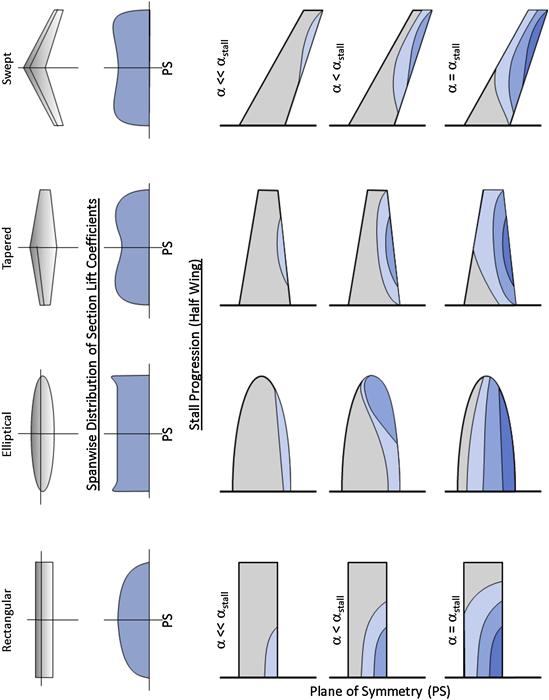


FIGURE 9-73 Stall progression on straight tapered wing planforms differing in AR, λ, washout, and surface roughness. (Based on Refs [39–41])
Another example is depicted in Figure 9-74, which compares the progression of the separation region on untwisted elliptical and crescent-shaped wing planform shapes, based on a paper written by van Dam, Vijgent, and Holmes [43], showing how the stall progression can be highly affected by vortical flow forming along a highly swept outboard leading edge. In the paper, the authors indicate that the separation-induced vortex flow over the highly swept tips of the crescent wing improved its stall characteristics when compared to the unmodified elliptical wing (whose stall characteristics were shown to be abrupt and unsteady). This viscous phenomenon delayed full stall of the experimental wing to a higher stall AOA (14.5° versus 13.0° for the elliptical wing) and yielded a higher CLmax (1.06 versus 0.98, respectively). At lower AOA, the lift characteristics were found to be practically identical, something important to keep in mind for cruise operations. The complex surface flow depicted in Figure 9-80 shows that at 14° the outboard portion of the elliptical wing is fully separated, while it is mostly attached on the crescent wing. The crescent-shaped wing planform is reminiscent of that of numerous species of birds.
FIGURE 9-74 Stall progression on a crescent-shaped and an elliptical wing planform of comparable geometry shows the complex flow inside a separation region. (Based on Ref. [42])
9.6.4 Tailoring the Stall Progression
Good stall characteristics are simply a question of safety. An airplane that constantly rolls left or right at stall is at an increased risk of entering spin. If the airplane stalls close to the ground, perhaps as a consequence of the pilot banking hard to turn on final approach, there simply is no time (or altitude) to recover, no matter how good spin recovery characteristics the airplane has or how proficient the pilot. The consequence is usually a fatal crash.
There is no good reason to develop an airplane without good stall characteristics, especially considering these can be tailored into the airplane from its inception. It is not being claimed that this is easy, although nowadays it is easier using CFD solvers. CFD methods such as vortex-lattice, doublet-lattice, and other panel codes can be used to determine the distribution of section lift coefficients along the span of the aircraft, even though such solvers ignore viscosity. Navier-Stokes solvers can be of even greater use, as long as the selected turbulence model does not mislead the user in the extent and shape of the flow separation (for instance, see Section 23.3.16, Reliance upon analysis technology). Then, armed with an understanding of how the stall progresses along the wing, the designer can select a combination of airfoil types and wing washout to control the stall progression along span of the wing.
Design Guidelines
The target stall pattern should always begin at the root and progress toward the tip as the AOA is increased. This ensures the wingtips will be the last part of the wing to stall, providing vital roll stability and control throughout the maneuver. If inviscid design methodology is used to tailor the stall progression, the goal should be to ensure the section lift coefficient (Cl) at the 70% span station is no higher than the maximum lift coefficient (Clmax) of the airfoil at that station. Furthermore, from 70% to 100%, Cl should gradually fall to zero. Some authors (e.g. Torenbeek [44]) recommend (Clmax − 0.1), but this may be hard to achieve in practice without excessive washout. At any rate, the idea is to promote roll stability at stall and washout is a powerful tool to provide this function. If a viscous analysis method is used (e.g. Navier-Stokes solvers), then a more pinpointed tailoring can be accomplished, but only if the flow separation prediction is deemed trustworthy. For something as serious as stall tailoring, flow visualization of the separated region obtained from wind tunnel testing should always be used to validate the CFD model.
Figure 9-75 shows an example of typical linear analysis for a tapered wing (λ = 0.5) that features the same airfoil (NACA 652-415) throughout the wing. Since the Reynolds number at the tip is only one-half of the root value, the Clmax is less at the tip and this should be taken into account for airplanes that feature tapered planform shapes. The baseline wing design (solid curve) has no washout, whereas the other three have a 2°, 4°, and 6° washout, respectively. The graph shows the distribution of Cl for these four models at AOA of 16°. The thick dashed line shows the distribution of the Clmax from root to tip.

FIGURE 9-75 The effect of washout on probable stall progression. The baseline wing is more tip-loaded than the ones with washout and this will cause it to stall closer to the wingtip, which may cause roll-off problems. Washout is a powerful means to control stall progression and can be enhanced by selecting a high-lift airfoil at the tip.
The graphs in Figure 9-75 show that the Cl for the baseline wing exceeds the Clmax between Spanwise Station 0 to about 0.87. This means the wing should be expected to be fully stalled to that point, something that would result in poor stall characteristics, as barely 10% of the span (at the tip) is un-stalled. The proposals for a 2°, 4°, and 6° washout all lead to improvements, especially the last one (6°), which brings the stall to Spanwise Station 0.65. However, as can be seen in Table 9-6, washout higher than 4° is rare. Excessive washout can lead to an increase in the lift-induced drag as the wing must be operated at a higher AOA to generate the same airplane lift coefficient (CL). A better solution would be to feature less washout, say somewhere between 2° and 4°, and feature a tip airfoil that has a higher Clmax than the root (an aerodynamic washout). Of course it is assumed such an airfoil would offer gentle stall characteristics (not those of the NACA 23012 airfoil presented in Section 8.2.10, Famous airfoils).
Tailoring Stall Characteristics of Wings with Multiple Airfoils
A possible stall tailoring remedy is proposed in the graph of Figure 9-75. It consists of increasing the Clmax of the tip airfoil from 1.57 to about 1.7, by defining a new tip airfoil. Of course, this may pose some challenges; such an airfoil might possess some undesirable characteristics too. However, assuming this is achievable; it may be possible to manufacture the wing without a geometric washout. This can be an advantage for some composite wing designs, as it allows uni-directional plies in the spar to be laid up in a more manufacturing-friendly fashion than a twisted spar. In practice, however, tailoring the wing for good stall progression is solved using a combination of both geometric and aerodynamic washouts.
Other Issues Associated with Wings with Multiple Airfoils
Multi-airfoil wings are the norm for high-performance aircraft, but are also common in smaller and simpler GA aircraft. High-performance aircraft require wings that allow the airplane to operate at low airspeeds while avoiding compressibility effects associated with high-speed flight. It takes sophistication in manufacturing to produce such wings. This is particularly challenging in the production of wings made from alloys, as the difference in geometry inevitably requires the wing skin to be stretched to conform to the resulting compound surface. This will become clearer in a moment.
A hypothetical multi-airfoil wing is shown in Figure 9-76, Figure 9-77, and Figure 9-78, with the layout presented in Figure 9-76. It should be stressed there is no rhyme or reason why the particular airfoils have been selected other than to demonstrate aerodynamic, structural, and manufacturing complexities that may arise in such a wing design. The wing is defined using three airfoils: at the plane of symmetry (the “root”); at the intersection of the flap and aileron; and at the tip. Structurally, the intersection of the flap and aileron is a good location to anchor a new airfoil as a rib is required there to mount the hard-points for the control surfaces.
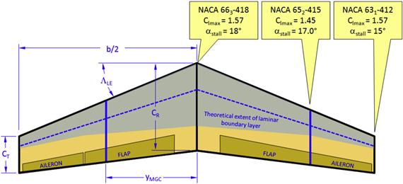
FIGURE 9-76 An example wing layout, showing the theoretical extent of laminar boundary layer and variation in its maximum lift capability.
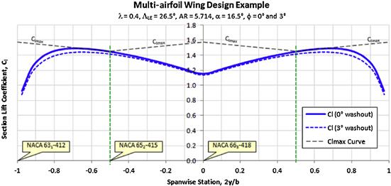
FIGURE 9-77 An example of a potential flow lift analysis of the multi-airfoil wing layout that features 0° and 3° washout.
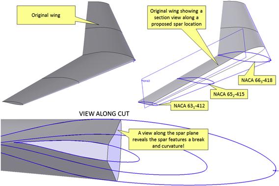
Figure 9-76 also shows that the airfoil selection will affect the extent of the laminar boundary layer on the wing’s upper surface (assuming this is achievable). This change must be accounted for in the drag estimation for the wing. Achieving a laminar boundary layer is difficult, as has already been discussed in Chapter 8, The anatomy of the airfoil. Attempting this on the above wing will require careful and more expensive manufacturing tooling.
Figure 9-77 shows the distribution of section lift coefficients along both wing halves at α = 16.5° and is based on potential flow analysis. It also shows how the maximum lift varies along the span because of the three airfoils and that the progression of stall begins just outside the 50% span station. Also plotted is the distribution of Cl for the same wing with a 3° washout, showing improvements, although the wing is still highly tip-loaded. The reader is also reminded that the linear method used does not correctly predict flow separation due to chord- and spanwise flow (recall this is a swept wing design). Therefore, although the linear method is helpful in understanding the airflow around the wing, ultimately the graph represents an ideal flow scenario that is not present in the real flow.
Figure 9-78 shows some structural and manufacturing issues that present themselves in wings with multiple airfoils. The geometry that results often comes as a surprise to novice engineers designing the structure of such wings. Since the three airfoils used have dissimilar geometry, the spar extending from root to tip will be subject to a geometric non-linearity; the skin will form a compound surface. In the figure, the wing is cut along a proposed spar-plane. The view along the cut shows two situations are present: first, there is a discontinuity in the spar OML at the mid-span station. Second, mathematically, the spar cap must also feature a slightly curved surface, extending from root to midspan and then to the tip. If it is required that the skin must adhere perfectly to the compound surface and it will be made from aluminum, the sheet metal for the spar and skin will have to be pressed to shape using hydraulic presses. This will greatly increase the cost of production. In real aircraft, especially less expensive ones, the discontinuity is usually solved by sheets terminating along the discontinuity. The curvature may have to be solved by straightening the spar cap and accepting that the wing will not be what the aerodynamics group really wants or by inserting shims between the spar and the skin. This may also make it more challenging to achieve a laminar boundary layer, as the resulting shape may no longer present the intended theoretical shape.
9.6.5 Cause of Spanwise Flow for a Swept-back Wing Planform
Swept-back wings can experience a significant and uncontrollable pitch-up moment at high angles-of-attack. The reason for this is twofold:
(1) The aft-swept planform induces local upwash near the tip which increases the local section lift coefficients. This means that the tip airfoils reach their stall section lift coefficients sooner than the inboard airfoils.
(2) Air begins to flow in a spanwise direction near the tip, but this leads to an early flow separation.
The first cause is somewhat hard to explain in layman’s terms, but we will try. Imagine the wing is cut into a finite number of small sections along the span of the wing. The sections extend from the root to the tip such that the inboard section is always upstream of the adjacent outboard section. For this reason, the inboard section will begin to disturb the flowfield before the section outboard of it. A part of this disturbance is an upwash ahead of that section which extends spanwise into the flowfield. Then, when the outboard section begins to disturb the flowfield ahead of it, there is already an upwash component in it, induced by the section inboard of it. This section will then impart it own influence on the flowfield, which manifests itself as a slightly greater upwash for the section outboard of it, and so on. The upwash implies a greater local AOA. A greater local AOA implies a higher section lift coefficient.
The cause of the spanwise flow, on the other hand, and which is the topic of this section, can be explained as follows. Consider the swept-back wing of Figure 9-79, which shows an aircraft with a swept-back wing at some AOA. Two sample chordwise pressure distributions are drawn on the right wing. Also, the locus of the peak spanwise pressure distribution along the wing is shown as the dotted curve drawn at the pressure peaks. It can be seen that the pressure peak on the outboard wing is higher than inboard. Now, consider a line perpendicular to the centerline of the fuselage at some arbitrary chord station. It cuts through the chordwise pressure distributions as indicated by the vertical arrows. The inboard arrow is shorter than the outboard one, indicating higher pressure than on the outboard one (remember these distributions represent low and not high pressures). For this reason the higher pressure on the inboard station forces air to flow from the inboard to the outboard station, giving the flow field an overall outboard spanwise speed component. This is shown as the streamlines on the left wing.
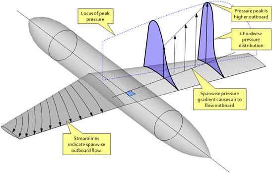
FIGURE 9-79 The spanwise pressure gradient on an aft-swept wing results in an outboard spanwise flow. The opposite holds true for a forward swept wing. (Based on Ref. [17])
9.6.6 Pitch-up Stall Boundary for a Swept-back Wing Planform
As stated in the previous section, swept-back wings suffer from significant pitch-up moment near and at stall. The effect depends on the quarter-chord sweep angle, ΛC/4, and aspect ratio, AR. The effect is investigated in NACA TR-1339 [45] and NACA TN-1093 [46]. Figure 9-80 is reproduced from those references and summarizes the effect. It shows that the higher the AR, the less is the ΛC/4 at which the pitch-up is experienced. This is very important in the development of long-range high-subsonic aircraft as a high AR favors long-range but high ΛC/4 favors high airspeed. These properties are therefore mutually detrimental. As contemporary airliners demonstrate, the development of the modern airfoil has remedied this limitation with its greater critical Mach number (at which shocks begin to form). This has allowed aircraft with lower ΛC/4 (≈ 20°–27°) to utilize higher AR and, thus, operate more efficiently at the usual cruising speeds of such aircraft (M ≈ 0.78–0.82).
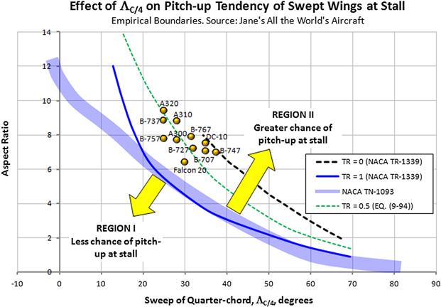
FIGURE 9-80 Empirical pitch-up boundary for a swept-back wing. Reproduced based on Refs [44] and [45].
An empirical equation based on the data in Ref. [44] can now be developed. It relates the taper ratio, λ, and, sweep angle of the quarter chord in degrees, ΛC/4, to calculate an AR limit for swept-back wings. For a given ΛC/4 the selected AR should be less than this limit:
![]() (9-94)
(9-94)
Alternatively, given a target AR, the ΛC/4 in degrees should not exceed the value below:
![]() (9-95)
(9-95)
As shown in Figure 9-81, the combination of AR, λ, and ΛC/4 can lead to desirable or undesirable results in terms of nose pitch-down or pitch-up characteristics at stall. Aircraft that feature aft-swept wings should always be wind tunnel tested for stability at stall, but the awareness of the data used to produce Figure 9-80 can go a long way in preventing serious stall problems from presenting themselves.
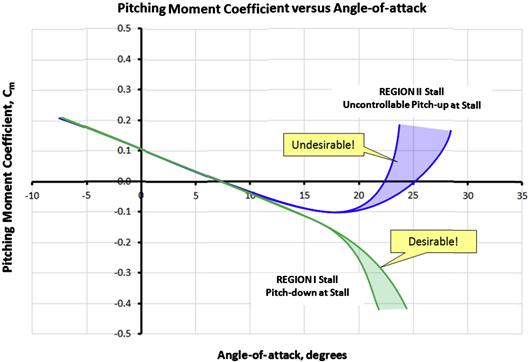
FIGURE 9-81 The combination of AR, TR, and quarter-chord sweep can lead to desirable or undesirable pitch characteristics at stall.
Finally, NACA RM-L8D29 [47] presents various results that are helpful to the designers of swept-back wings. It investigated the effect of a number of high-lift devices and fences on the stall characteristics on stall characteristics (see Figure 9-82). It concluded that the half-span, leading-edge slats eliminated the tip stall and prevented the nose-up pitching moment. The flaps complicated the stall characteristics and formed a loop in the pitching moment curve (in the figure), although it was suggested it could be brought under control using an appropriately stabilizing surface.

FIGURE 9-82 The effect of various combinations of a double-slotted flaps and slats on the pitching moment of a 37° swept wing. The loop is attributed to the section characteristics of the double-slotted flap. (Based on Ref. [46])
Derivation of Equations (9-94) and (9-95)
The derivation is based on the data obtained using Ref. [44], which presents two curves that are functions of the quarter-chord sweep angle, ΛC/4; one represents a taper ratio λ = 0 and the other λ = 1. The idea is to derive an empirical expression that is a function of λ and ΛC/4 that closely fits both expressions. This can be done with some numerical analysis. A least-squares exponential fit to the two curves yields the two following expressions:
![]()
![]()
Since the values of the two exponents are relatively close to each other it can be deduced that the value of λ has minimal impact on it and primarily affects the constant. For this reason the average of the two (−0.04267) can justifiably be used for the empirical expression. Assuming a function of the form:
![]() (i)
(i)
The function f(λ) can then be approximated by noting that the constant changes from 35.885 when λ = 0 to 18.171 when λ = 1. It is convenient to employ a parametric representation for this variation, in particular considering that λ can be used unmodified as the parameter. Thus, Equation (i) can be rewritten as follows:
![]() (ii)
(ii)
And this is Equation (9-94). Equation (9-95) is simply obtained by solving for ΛC/4.

QED
9.6.7 Influence of Manufacturing Tolerances on Stall Characteristics
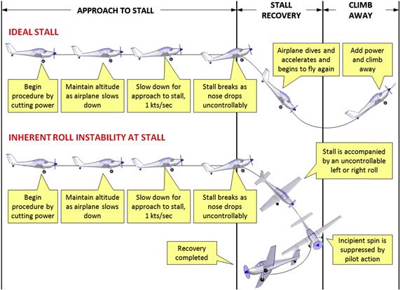
Inherent roll instability at stall is one of the most common handling deficiencies affecting aircraft. In fact, most aircraft ever built have displayed the condition to some extent, requiring the introduction of “fixes” to remedy it. The manifestation of this condition occurs at stall as the aircraft does not drop the nose with wings level, but rather rolls uncontrollably to the left or right side (see Figure 9-83). Its root causes are complicated and one should not assume there is a single cause, but rather a combination of factors.
It may sound strange, but all aircraft are inherently asymmetric, even though this is usually impossible to discern with the naked eye. Nevertheless, every single serial number differs slightly from the previous or the following one in its deviation from the intended outside mold line (OML). Not even the left wing of any given airplane is a perfect mathematical mirror image of the right one, although it is completely invisible to the casual observer. There are always subtle differences in washout, thickness, waviness, and their corresponding locations on each wing, all of which may combine to promote roll instability at stall.
A typical deviation from the OML in the aviation industry amounts to ±0.125 inches, although most wings must usually meet tolerances ranging from ±0.050 to ±0.100 inches over the lifting surfaces. Manufacturers of GA aircraft that feature NLF lifting surfaces often take it one step further and maintain even tighter tolerances; sometimes as tight as ±0.005 inches along the leading edge. While maintaining tolerances is imperative in the manufacture of aircraft, overly tight tolerances are of detrimental value. They call for expensive and robust inspection procedures and additional manpower to demonstrate such wings meet the set specifications. Very tight tolerances should always be justified with research.
One of the main concerns manufacturers have with NLF wings is their sensitivity to deviations from the OML, as this may promote early transition of a laminar boundary layer into a turbulent one, which, in turn, increases drag. This often requires expensive repairs to be made to wings that arguably are just fine. The author of this book once investigated the some 300 production aircraft with NLF wings to determine whether there was a correlation between the magnitude of such small manufacturing deviations and stall characteristics reported by the production flight test pilots. No correlation could be found. Tight tolerances had subjected the production to costly inspection procedures without measurable benefits.
While this is not intended to reject the application of tight tolerances in the manufacturing of NLF wings, there clearly is a point of diminishing returns. It turns out that near stall AOA, the flow is altogether separated anyway and, therefore, insensitive to minor deviation from the OML. The source of roll instability should be looked for elsewhere, such as in deviation in thickness, twist, dihedral, and objects that are asymmetrically exposed to the airflow.
It would seem from the above discussion that if too tight tolerances are a problem, then perhaps loose tolerances may be desirable. However, this is not the case. Loose tolerances allow an airplane to be excessively asymmetric, not just in surface qualities, but in large deviation from the OML of the surface that almost certainly would cause an inherent roll instability. It is best to design sensitivity to small deviations out of the OML by providing assertive aerodynamic roll stability at high AOA. This can be done by increasing the camber of the wingtip airfoil (by specifically selecting a high-lift airfoil), or by reducing its AOA using washout, or by providing a leading-edge extension (see Section 23.4.11, Stall handling – wing droop (cuffs, leading-edge droop), or by introducing slats.
9.7 Numerical Analysis of the Wing
The advent of the digital computer has clearly revolutionized science and engineering. As far as aircraft design is concerned, the technology allows far more complicated and realistic analyses to be performed than previously possible. In its most sophisticated form, the use of computer technology allows the full Navier-Stokes equations (NSE) to be solved for extremely complex situations. This ranges from airflow resembling that experienced by an insect to that of a tumbling meteorite entering Earth’s atmosphere at hypersonic speeds. At the present time, however, the application of this method is both time-consuming and expensive as it requires a detailed digital model of the geometry to be prepared and flow solution obtained using a cluster of interconnected computers. Meshing the model is often more art than science and requires an experienced individual to complete. Improperly designed mesh simply yields erroneous results. This is further compounded by the amount of time required to solve the problem. It can easily take a couple hours to a couple of days to accomplish, depending on the complexity of the body and the computational prowess of the individual (or company) involved. For this reason, conceptual design using NSE solvers is very impractical and should not even be considered. Currently, NSE is really a post-conceptual design tool; it should be used after the concept has been designed and not to design it.
There are a number of practical numerical methods available to the designer that, in comparison, are lightning fast and, for attached flow, are equally as accurate as the solution obtained using the NSE. Among those are the lifting line method and panel methods such as the vortex-lattice or doublet-lattice. While programmatically considerably older than the modern Navier-Stokes solver, they remain far more practical during the conceptual design phase and are simple enough to implement using a desktop computer. Due to space limitations, only the most basic of these methods will be demonstrated; Prandtl’s lifting line method. For other methods, the reader is directed toward excellent texts such as those by Katz and Plotkin [48]; Pope [49]; Bertin and Smith [50]; and Moran [51].
9.7.1 Prandtl’s Lifting Line Theory
Developed by Ludwig Prandtl (1875–1953) and his colleagues at the University of Göttingen between 1911–1918, the lifting line theory can be used to determine the aerodynamic characteristics of straight three-dimensional wings. The method does not treat wings with dihedral or sweep, but can account for wing twist and varying airfoils and chords along the span of the wing. It is reliable for wings whose AR is no smaller than about 4. The method mathematically replaces the wing with a number of constant-strength vortices, here denoted with the Greek letter Γ. The problem, effectively, revolves around determining their strength; however, once this has been accomplished, it is possible to estimate a number of characteristics, such as lift and drag, downwash, and distribution of lift along the wing. It is thus useful not only for aerodynamic properties, but also for structures and stability and control. A derivation of the method will now be presented, but first the following mathematical constructs must be introduced.
The Vortex Filament and the Biot-Savart Law
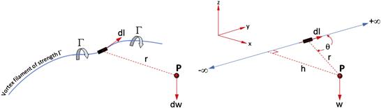
A vortex filament is an imaginary spatial curve that induces a rotary flow in the space through which it passes (see Figure 9-84). The best analogy is to think of it as the center of a tornado with the associated circulatory flow around its core. The ability of the filament to induce circulation around it depends on its strength, denoted by Γ. Consider an infinitely small vector segment dl along the filament and some arbitrary point P in space. The small segment will induce a velocity dw at the point P, whose magnitude can be determined using the Biot-Savart4 law:
The Biot-Savart law is named after the French mathematician and physicist Jean-Baptiste Biot (1774–1862) and Félix Savart (1791–1841), a fellow Frenchman who trained for a career in medicine, although his mind was absorbed by natural philosophy.
The derivation of the law is beyond the scope of this book, but interested readers can refer to almost any textbook on electrical engineering. The law was actually derived to relate a magnetic field induced by an electric current in a wire, but it can also be used to estimate the circulation of flow around a wing. This is because the Biot-Savart law is one of numerous solutions of Laplace’s equation, which is the governing equation for irrotational, incompressible fluid flow. It is shown below for convenience:
![]() (9-97)
(9-97)
where ϕ is the velocity potential. Note that the direction of the velocity is imperative. In accordance with a right-handed coordinate system, assume the thumb of the right hand to point in a direction indicated by the filament dl in Figure 9-84. Then the other four fingers curl around the filament as if holding a rope. The direction of the velocity is always in the direction the four fingers make. This is an important concept to keep in mind for what follows.
In the development of the lifting-line theory, we will be applying the Biot-Savart law to a number of straight (versus curved) vortex filaments that are infinitely long. Such a straight segment is shown in Figure 9-84. It stretches from −∞ to +∞. Knowing the contribution of the tiny segment dl, the total velocity induced at the point P can be determined by integrating the contribution along the entire filament, i.e.:
 (9-98)
In order to constrain the discussion here to the bare essentials, the solution of the integral is omitted and only the final result presented. The interested reader can, for instance, refer to Anderson [52] for the evaluation. The solution involves relating the parameters h, r, and θ in Figure 9-84, and inserting into the integral prior to its evaluation. Thus, the fluid speed at the point P, induced by the straight vortex filament of strength Γ, is given by:
Helmholz’s Vortex Theorems
In 1858, the German scientist Hermann von Helmholz (1821–1894) made the next step by using the vortex filament to analyze inviscid, incompressible fluid flow. In doing so he established what has become known as Helmholz’s vortex theorems. These state that:
(1) The strength of the vortex filament is constant along its entire length; and
(2) A vortex filament cannot end in a fluid, but must either extend to infinity or form a closed path.
These theorems are used to evaluate a special kind of vortex called a horseshoe vortex. The horseshoe vortex has important properties that will be discussed shortly and that allow it to be used to represent the lift of a finite wing.
Lifting Line Formulation
Now that we have established that a straight vortex induces a circulation around the vortex filament, it is possible to extend the idea to a three-dimensional wing. An observation of real finite wings reveals two important facts:
(1) The wing induces circulation that extends from tip to tip; and
(2) Each wingtip sheds a vortex that extends far into the flow field behind the wing.
This fact can be approximated using three separate vortex filaments as shown in Figure 9-85. First, a trailing vortex extends from infinity to the left wingtip. Then, a bound vortex extends from the left wingtip to the right wingtip. And finally, a third trailing vortex extends from the right wingtip back to infinity. This system of vortices not only satisfies Helmholz’s vortex theorems, it also induces a flow field that resembles that of real three-dimensional wings. Additionally, the three vortices, which are of a constant strength Γ, all have the same sign, as can be observed using the right-handed rule (the thumb of the right hand should point forward for the first vortex, to the right for the second one, and backward for the third one).
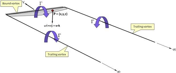
FIGURE 9-85 The flow field around a wing approximated by three connected constant-strength straight vortex filaments. On the wing plane, u = v = 0.
While promising, there is a problem with this system in that it leads to a spanwise lift distribution that is constant. However, this implies that the lift at the wingtips is non-zero, but this is physically impossible. In fact, a single vortex like this will cause the downwash at the wingtip to go to infinity. The solution to this dilemma is to add more horseshoe vortices to the system, each of lesser span than the next, and with its own constant circulation (see Figure 9-86). The inboard vortices usually have greater strength than the outboard ones, but the interaction of all of them causes the resulting downwash to resemble that shown by experiment. This way, the strength of each individual vortex will be constant, but their total interaction along the span will result in a variable spanwise load distribution.
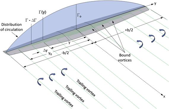
The lifting line method is based on the assumption that the vortex strength along the span is known. Consider that, at some spanwise wing station y, the vortex strength is given by the value Γ(y). This means that if we move a distance Δy to another spanwise station, the change in the strength of the vortex, ΔΓ, can be found from:
![]() (9-100)
(9-100)
Now consider the spanwise station at y0 and the vortex at y, shown in Figure 9-86. It is possible to determine the downwash (i.e. the vertical speed) induced at y0 by the vortex at y (see depiction in Figure 9-87). Let’s denote the contribution to the total downwash at y0 by ![]() . Since the trailing vortex extends from infinity to x = 0 where it stops (because that is where we have planted our vortex system, so it does not extend to −∞ also), the influence will be half of that shown by Equation (9-99), or:
. Since the trailing vortex extends from infinity to x = 0 where it stops (because that is where we have planted our vortex system, so it does not extend to −∞ also), the influence will be half of that shown by Equation (9-99), or:
![]() (9-101)
(9-101)
Note that as depicted in Figure 9-86 and Figure 9-87, the vortex at y will induce an upward pointing contribution at y0. This is emphasized by the + sign in the equation. In order to calculate the total downwash at y0 due to all the vortices distributed along the span, Equation (9-101) is integrated from the left wingtip (y = −b/2) to the right one (y = +b/2):
 (9-102)
As can be seen, the downwash will ultimately depend on the strength of the circulation along the span. The contributions of other vortices in the system eventually yield a downward-pointed velocity at y0. With the downwash at y0 known, the downwash angle ![]() at y0 can now be calculated as follows:
at y0 can now be calculated as follows:
![]() (9-103)
(9-103)
where V denotes the far-field airspeed. As stated in Section 15.3.4, The lift-induced drag coefficient: CDi, the downwash behind the wing and corresponding upwash in front of it effectively “tilt” the undisturbed air through an induced AOA, denoted by αi, reducing the geometric angle-of-attack, α, at the quarter-chord by a magnitude, to what is called the effective AOA, αe (see Figure 9-88):
![]() (9-104)
(9-104)
Note that if the wing features washout, αi and thus αe become a function of the spanwise station. Similarly, cambered airfoils are treated by subtracting the angle of zero lift from the geometric AOA. The presence of the induced AOA tilts the lift force back by the angle ε (see Figure 15-20) and must therefore be resolved into two force components: one normal to the flight path (lift) and the other parallel to the flight path (lift-induced drag). The Kutta-Joukowski theorem (see Section 8.1.8, The generation of lift) makes it possible to calculate these two forces per unit span using the following expressions:
![]() (9-105)
(9-105)
Lift-induced drag per unit span:
![]() (9-106)
(9-106)
The minus sign is necessary to ensure the negative value of the downwash produces a positive drag force. The total lift and lift-induced drag forces can now be determined as shown below:
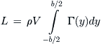 (9-107)
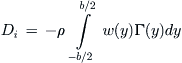 (9-108)
Consequently, the lift and lift-induced drag coefficient are given by:
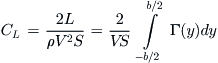 (9-109)
Lift-induced drag coefficient:
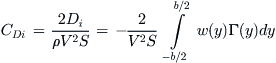 (9-110)
If there is a representative zero-lift AOA for the wing, the lift curve slope can be calculated from:
![]() (9-111)
(9-111)
The subsequent articles present several applications of this method.
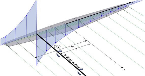

9.7.2 Prandtl’s Lifting Line Method – Special Case: The Elliptical Wing
As discussed in Section 9.4.4, Elliptic planforms, from a standpoint of efficiency the elliptical wing planform is very practical in aircraft design and is therefore of great interest to the aircraft designer. In this article, the lifting line method is applied to an elliptical planform and several useful closed-form solutions of selected aerodynamic characteristics are derived. These characteristics are helpful even if they are only used for comparison reasons. The solution assumes that the distribution of circulation is known and is given by:
![]() (9-112)
(9-112)
Using this distribution, the following aerodynamic characteristics for the elliptical planform can be derived (see derivation section that follows):
![]() (9-113)
(9-113)
![]() (9-114)
(9-114)
![]() (9-115)
(9-115)
![]() (9-116)
(9-116)
![]() (9-117)
(9-117)
![]() (9-118)
(9-118)
Lift-induced drag coefficient:
![]() (9-119)
(9-119)
Derivation of Equations (9-113) through (9-119)
First evaluate the derivative dΓ/dy. This can be done using the chain rule of differentiation:

This can be used with Equation (9-102) to calculate the total downwash at any spanwise station, say y0 (for the sake of consistency):

It is helpful to evaluate the integral by transforming spanwise stations into an angular form as follows:
![]() (9-120)
(9-120)
Using this transformation, we find the lower limit (-b/2) becomes 0 and the upper one (+b/2) becomes π. If we define ![]() the above integral can be rewritten as follows:
the above integral can be rewritten as follows:

Simplifying further yields:
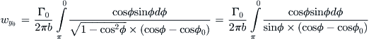
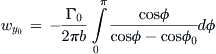
The evaluation of this integral is beyond the scope of this text, but a solution is provided in Karamcheti [53]. An alternative solution method based on the original expression omitting the transformation is presented by Bertin and Smith [50]. In either case, the resulting expression reduces to:
![]() (ii)
(ii)
This is Equation (9-114). Note that the distribution of downwash is constant along the span. The downwash angle can thus be obtained from Equation (9-103):
![]() (iii)
(iii)
This is Equation (9-115). Note that this angle is constant along the span as well. Inserting Equation (9-112) into (9-107) yields the total lift generated by the wing:
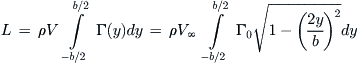 (iv)
(iv)
Using the above angular transformations, Equation (iv) can be rewritten and simplified as follows:

This is Equation (9-116). The lift coefficient can now be determined from:
![]() (vi)
(vi)
This is Equation (9-118). Alternatively, the vortex strength Γ0 is readily obtained from Equation (vi) as follows:
![]() (vii)
(vii)
This is Equation (9-113). Similarly, the lift-induced drag can be computed from Equation (9-108):
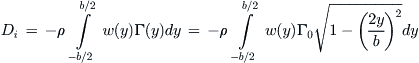 (viii)
Inserting Equation (9-114) and using the spanwise angular transformation of Equation (9-120), we get Equation (9-117):
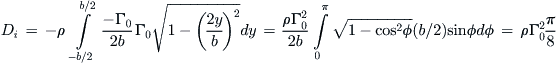 (ix)
(ix)
The lift-induced drag coefficient can now be determined as follows, using Equation (vii):
![]() (x)
(x)
This is Equation (9-119).
QED
9.7.3 Prandtl’s Lifting Line Method – Special Case: Arbitrary Wings
The history of aviation reveals that most aircraft do not feature elliptical wing planform shapes. It follows that it is desirable to extend the lifting line method to non-elliptical wings. One way of accomplishing this is to represent the spanwise distribution of vortex strengths using a Fourier sine series, consisting of N terms:
Fourier series lift distribution:
![]() (9-121)
(9-121)
Note that if the lift distribution is symmetrical, all even values of n are omitted. The first equation of interest is the one that allows the coefficients A1, A2, A3, …, AN to be solved.
![]() (9-122)
(9-122)
The monoplane equation is used to construct a system of simultaneous equations, as shown below. The left-hand side of this equation is called the aerodynamic influence matrix:
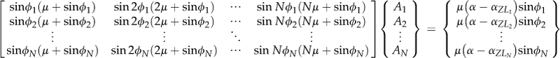 (9-123)
where
αZLi = zero lift angle for the airfoil at station ϕ
ϕi = angles (in radians) that correspond to the spanwise angular stations obtained from ![]() (i.e. Equation [9-120]), in radians
(i.e. Equation [9-120]), in radians
![]() , dimensionless; the airfoil’s lift curve slope,
, dimensionless; the airfoil’s lift curve slope, ![]() , may be a function of ϕ
, may be a function of ϕ
Solving the system leads to a number of interesting results, some of which are presented below.
![]() (9-124)
(9-124)
![]() (9-125)
(9-125)
![]() (9-126)
(9-126)
The lift curve slope can thus be calculated from:
![]() (9-127)
(9-127)
And lift-induced drag coefficient:
![]() (9-128)
(9-128)
where ![]() and
and ![]() .
.
As stated above, if the spanwise distribution of lift is symmetrical, all the even indexed constants (A2, A4, …) of the summation are set to zero. This can be written as follows:
![]() (9-129)
(9-129)
See Figure 15-22 for a graph plotting δ as a function of taper ratio and aspect ratio for straight tapered wings.
Change in Induced Angle-of-attack
The induced AOA on an arbitrary planform differs from that of an elliptical planform of an equal AR according to the following expression:
![]() (9-130)
(9-130)
where τ is given by:
![]() (9-131)
(9-131)
Derivation of Equations (9-124) through (9-128)
In order to determine the coefficients A1, A2, A3, …, AN, the circulation for the N vortices must be determined. The procedure begins by relating the section lift coefficient at any angular station ϕ as follows:
![]() (i)
(i)
where C(ϕ) is the chord at a specific angular station ϕ. However, if the lift curve slope, ![]() , of the airfoil at the angular station ϕ is known, the section lift coefficient can also be determined from:
, of the airfoil at the angular station ϕ is known, the section lift coefficient can also be determined from:
![]() (ii)
(ii)
where ![]() is the zero-lift AOA of the airfoil at the angular station ϕ. Note that α, αZL, and αi are all functions of the angular station ϕ. By equating Equations (i) and (ii) we get:
is the zero-lift AOA of the airfoil at the angular station ϕ. Note that α, αZL, and αi are all functions of the angular station ϕ. By equating Equations (i) and (ii) we get:
![]() (iii)
(iii)
The term ![]() is given by Equation (9-102):
is given by Equation (9-102):
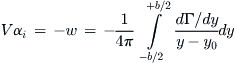 (iv)
(iv)
where the minus sign indicates a downward flow of air. Using the definition of ![]() given by Equation (9-121) this can be rewritten as follows:
given by Equation (9-121) this can be rewritten as follows:
![]() (v)
(v)
Therefore, Equation (iii) can be rewritten as follows:
![]() (vi)
(vi)
Expanding by inserting ![]() per Equation (9-121) yields:
per Equation (9-121) yields:
![]() (vii)
(vii)
Let ![]() and insert into Equation (vii). This leads to:
and insert into Equation (vii). This leads to:
![]()
Simplify terms in the summation sign to yields a governing equation that is called the monoplane equation.
![]() (9-122)
(9-122)
This equation yields a set of equations that must be solved simultaneously to obtain the constants A1, A2, A3, …, AN. The angle ϕ refers to a spanwise angle transformation of Equation (9-120). If the problem deals with symmetrical load distribution, all even terms (n = 2, 4, etc.) are omitted from the solution.
Next consider the lift coefficient generated by the wing, given by:
 (viii)
Again using the definition of ![]() given by Equation (9-121), Equation (viii) becomes:
given by Equation (9-121), Equation (viii) becomes:

The integral can be solved noting that:
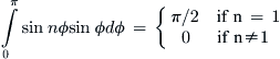
This allows Equation (ix) to be rewritten as follows:
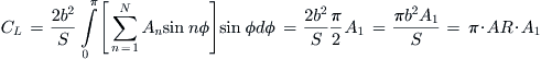 (ix)
(ix)
This is Equation (9-126). Then consider the lift-induced drag coefficient generated by the wing. Equation (9-108) defines the lift-induced drag, Di. Inserting Equation (v) for w(y) and Equation (9-121) for ![]() we get:
we get:

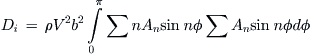
Where the evaluation of the integral yields:
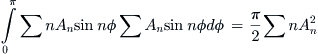
Therefore, the lift-induced drag is given by:
![]() (x)
(x)
Using Equation (9-110) it is now possible to determine the lift-induced drag coefficient:
![]() (xi)
(xi)
Since ![]() it is possible to rewrite this as follows:
it is possible to rewrite this as follows:
![]() (xii)
(xii)
This is a classic form of this equation, typically written in the following form, using the term δ to denote the lift-induced drag factor.
![]() (xiii)
(xiii)
It is evident that the minimum CDi is obtained when δ = 0, but this represents an elliptic lift distribution.
QED
Derivation of Equation (9-130)
Consider a two-dimensional airfoil and three-dimensional wing whose cross-sectional geometry is that of the said airfoil. The airfoil is akin to a three-dimensional wing of infinite wingspan. Consider these at specific AOA such that they both generate an equal lift coefficient, CL. This allows the aerodynamic AOA5 for each “wing” to be determined as follows:
This represents the difference in AOA between the two geometries. Next, insert ![]() into the expression for the three-dimensional wing, i.e.
into the expression for the three-dimensional wing, i.e. ![]() . This yields the following relationship between CLα and A1:
. This yields the following relationship between CLα and A1:
![]()
Replacing the corresponding term in the above equation for the difference in AOA leads to:
![]()
QED
EXAMPLE 9-13
Estimate the aerodynamic characteristics of the SR22 wing planform (ignoring the presence of the fuselage) using the lifting line method. Determine this using four terms in the monoplane equation, assuming symmetrical lift distribution. Assume the aircraft is flying at an AOA of 5° (0.08727 radians) and that the wing uses the NACA 65-415 airfoil (see Figure 9-60). Assume the airfoil’s zero-lift AOA, αZL, is approximately −2.7° (−0.04712 radians) and its lift curve slope, Clα, is 2π. Note that the dimensions in Figure 9-89 are calculated based on the geometry shown and are not the “official” numbers (e.g. official S = 144.9 ft2 and AR = 10). Determine the airspeed that the airplane must fly at S-L if it weighs 3400 lbf.
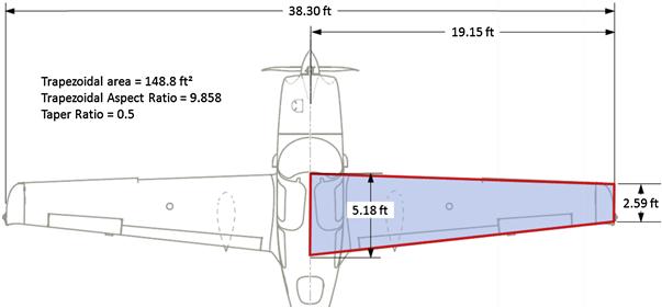
Solution
Begin by creating the relationship between the physical and angular span stations (see Figure 9-90). Note that the physical stations are given by ![]() (Equation [9-120]). For this reason, the cosine of ϕ is in effect a parameter that varies between 1 and 0 that can be used with a parametric representation for the chord. Thus, the chord at any spanwise station can be calculated from the following parametric equation:
(Equation [9-120]). For this reason, the cosine of ϕ is in effect a parameter that varies between 1 and 0 that can be used with a parametric representation for the chord. Thus, the chord at any spanwise station can be calculated from the following parametric equation:
![]()
where Cr = 5.18 ft and Ct = 2.59 ft.
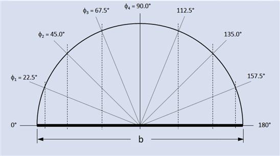
Next tabulate the following values:
Column ![]() and
and ![]() : contain the spanwise angular stations from Figure 9-90 both in degrees and radians.
: contain the spanwise angular stations from Figure 9-90 both in degrees and radians.
Column ![]() : contains the cosine of the angular station.
: contains the cosine of the angular station.
Column ![]() : contains the wing chord at the angular station. Calculated using
: contains the wing chord at the angular station. Calculated using ![]() .
.
Using the root and tip chords, Cr = 5.18 ft and Ct = 2.59 ft, respectively, this expression becomes:
![]()
Columns ![]() through
through ![]() : contain the various sines of the angular stations. These are needed to properly setup the matrix as required by the monoplane equation.
: contain the various sines of the angular stations. These are needed to properly setup the matrix as required by the monoplane equation.

Column ![]() : is calculated as follows, using values from the first row (ID = 1):
: is calculated as follows, using values from the first row (ID = 1):
![]()
Next prepare the aerodynamic influence matrix per Equation (9-123). Note that since the lift distribution is symmetrical, we are only concerned with the constants A1, A3, A5, and A7. This leads to the following setup.

For instance, the first row in the above matrix is calculated as follows, using the monoplane equation:
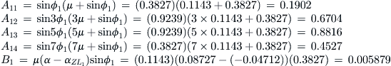
Solving the equations requires the square matrix to be inverted and then multiplied to the column matrix on the right-hand side, yielding the following values for the constants:
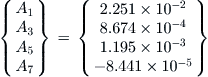
This allows the following aerodynamic parameters to be calculated. First, the lift coefficient can be calculated from Equation (9-126):
![]()
The lift-induced drag coefficient can be found by first determining the factor δ:
![]()
This yields the following drag coefficient per Equation (9-128):
![]()
Note that this value is for the wing without the detrimental effects of the fuselage. The lifting line method will always return efficiency that is too high for this reason. Finally, the wing’s lift curve slope can be determined as follows:
![]()
Finally, the airspeed the airplane must fly at in order to generate 3400 lbf of lift at 5° AOA can be determined as follows:
![]()
9.7.4 Accounting for a Fuselage in Prandtl’s Lifting Line Method
The lifting line method is seriously limited in that it applies directly to a “clean” wing; that is, the presence of a fuselage is not included. Consequently, the prediction will tend to return inflated span efficiencies, which can be detrimental to performance analysis. One way of correcting for this shortcoming is to consider only the exposed part of the wing. This is shown in Figure 9-91, which shows three wing planform shapes of equal spans, reference areas, and (therefore) AR. The top one is a “clean” elliptical wing, to which all other wings are compared when using the lifting line method. The wing in the center is a “clean” trapezoidal wing, whereas the bottom one is the same wing, except with a fuselage present. A schematic of the corresponding distribution of section lift coefficients is shown in the right portion of the figure.
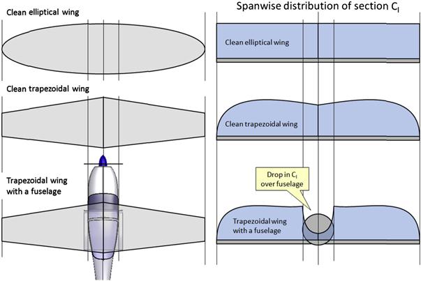
FIGURE 9-91 A schematic showing how the presence of a fuselage reduces the magnitude of the section lift coefficient over the fuselage.
It is evident from the preceding analysis that it compares the top (elliptical) and center wing (trapezoidal), whereas it would be more appropriate to compare the top and the bottom one. The fact that the fuselage so reduces the lift generated by the wing means that the airplane will have to fly at a higher AOA to make up for it. This is largely why the wing with the fuselage generates higher lift-induced drag than the clean wing and, when compared to the clean elliptical wing, reduces the Oswald span efficiency. The following method allows this to be taken into account when using the lifting line method, but first the following assumptions are introduced.
(1) Assume that the lift is entirely generated by the exposed wing panels and not by the region over the fuselage. This means that the section lift coefficients over the fuselage region are assumed to be zero.
(2) Assume that the fuselage acts as a wall. This allows the lifting line method to be applied to the exposed part of the wing by simply reducing the wing geometry as shown in Figure 9-92. For instance, the wingspan, b, will be reduced by the width of the fuselage, wfus.
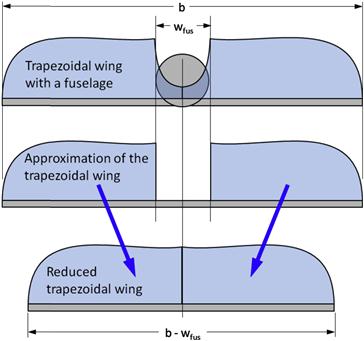
FIGURE 9-92 A schematic showing how the presence of a fuselage can be accounted for using the lifting line method.
![]() (9-132)
(9-132)
Let the planform area corresponding to the wing inside the fuselage be given by Cr × wfus. Therefore, the reduced wing area SR is given by:
![]() (9-133)
(9-133)
![]() (9-134)
(9-134)
Furthermore, reducing the wingspan will modify the taper ratio because the root chord changes. The reduced taper ratio can be estimated using a parametric representation for the chord:
![]()
This can be used to determine the reduced taper ratio, λR:
![]() (9-135)
(9-135)
So, rather than analyzing the complete wing, its wing span and area should be reduced using the above expressions. Therefore, the wing will now require a higher AOA in order to generate the CL required for a given flight condition.
EXAMPLE 9-14
Estimate the aerodynamic characteristics of the SR22 wing planform (including the presence of the fuselage) using the corrected lifting line method just discussed. Use all the information from Example 9-9 and assume a fuselage width of 50 inches (4.167 ft). Determine the CL required for the airplane to generate 3400 lbf at 98.4 KCAS and use this to estimate the aerodynamic characteristics. Then, compare it to that of Example 9-9 (the AOA and CL of Example 9-13 are 5° and 0.6971, respectively).
Solution
The procedure is identical to that of Example 9-13, so only results will be cited. First, compute the reduced wing parameters:
Then, estimate the CL required by the smaller wing:
![]()
Proceeding with the analysis method presented before, the results presented in Table 9-10 were obtained. It can be seen that while the “clean” wing requires 5° to lift 3400 lbf at 98.4 KCAS, the reduced wing (more realistic) requires 6.43° (see Table 9-10 below, where ‘original’ refers to the clean wing and ‘reduced’ refers to the wing with the fuselage). Consequently, its induced drag coefficient is 47% greater than the “clean” wing.
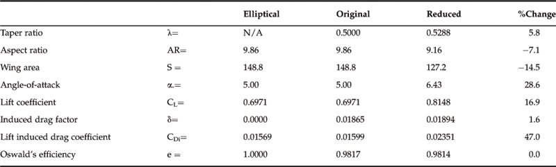
9.7.5 Computer code: Prandtl’s Lifting Line Method
The following code implements the lifting line method for an arbitrary wing using the above formulation. It is written using Visual Basic for Applications (VBA) and can be used as is in Microsoft Excel. It allows as many vortices as system resources allow to be used for the analysis, represented by the variable N (see the commented variable definitions in the code). A value of N larger than 50 is impractical; N in the ballpark of 10–14 is adequate in most instances.
In order to use the code and assuming Microsoft Excel 2007 is being used, the reader must select the Developer tab and then click on the Visual Basic icon to open a window containing the programming environment. This window will feature a title like Microsoft Visual Basic, followed by the filename, visible in the upper-left corner. In the project pane, typically docked at the left-hand side of this window, right-click to reveal a pop-up menu. One of the commands is the Insert command and it has a submenu indicated by a dark triangle. Hover with the mouse cursor over this triangle until the submenu appears. Select the Module command. This will open a VBA editor inside the main window. The program below must be entered there. The function is then called from the spreadsheet itself as shown in Figure 9-93. It can be seen that simple cell references are used to pass arguments to the routine. Here 50 vortices are being used, and the Mode is 2, which means that the term δ is returned.

Exercises
(1) Determine all the variables of the wing in Figure 9-94, if its planform area, S, is 200 ft2, AR = 7.5, and λ = 0.5. Approximate its internal volume if it features a constant 15% thick airfoil, whose maximum thickness is at 50% chord. If 30% of this volume is to be used for the fuel tanks, how much fuel can the wing hold and how much will it weigh assuming Jet-A fuel (1 US gal = 231.02 in3)?

Answer: b = 38.73 ft, Cr = 6.885 ft, MGC = 5.355 ft, YMGC = 8.607 ft, XMGC = 4.969 ft, ΛC/4 = 28.05°, ΛC/2 = 26.03°, wing volume is approximately 100 ft3; it can hold 225 US gallons, which weigh 1510 lbf.
Variables
| Symbol | Description | Units (UK and SI) |
| AOA | Angle-of-attack | Degrees or radians |
| AR | Aspect ratio | |
| ARcorr | Boosted aspect ratio | |
| ARe | Effective aspect ratio (AR · e) | |
| ARlim | Aspect ratio limit | |
| ARR | Reduced aspect ratio | |
| b | Wingspan | ft or m |
| bR | Reduced wingspan | ft or m |
| c | Chord length | ft or m |
| cavg | Average chord length | ft or m |
| cbhp | Specific fuel consumption of a piston engine | (lbf/hr)/BHP or g/J |
| Cd | Two-dimensional drag coefficient | |
| CD | Three-dimensional drag coefficient | |
| CDi | Lift-induced drag coefficient | |
| CDM | Compressibility drag coefficient | |
| CDmin | Minimum drag coefficient | |
| Cl | Two-dimensional lift coefficient | |
| CL | Three-dimensional lift coefficient | |
| CL0 | Zero AOA lift coefficient | |
| CLC | Average cruise lift coefficient | |
| CLmax | Maximum 3D lift coefficient | |
| CLmin | Minimum coefficient of lift | |
| Clp | Roll damping coefficient | |
| Clα | Two-dimensional lift curve slope | Per degree or per radian |
| CLα | Three-dimensional lift curve slope | Per degree or per radian |
| Cm | Two-dimensional pitching moment coefficient | |
| CM | Pitching moment coefficient | |
| CmROOT | Pitching moment coefficient of the root airfoil | |
| CmTIP | Pitching moment coefficient of the tip airfoil | |
| Cmα | Two-dimenstional pitching moment curve slope | Per degree or per radian |
| CMα | Three-dimensional pitching moment curve slope | Per degree or per radian |
| cr | Root chord length | ft or m |
| CrR | Reduced root chord length | ft or m |
| ct | Tip chord length | ft or m |
| ct | Thrust specific fuel consumption | 1/s |
| CY | Side force coefficient | |
| D | Drag | lbf or N |
| di(y) | Lift-induced drag per unit span | lbf/ft or N/m |
| dl | Infinitesimally small vector length | ft or m |
| dw | Velocity induced at arbitrary point P by dl | ft/s or m/s |
| e | Oswald’s span efficiency | |
| E | Endurance | s |
| h | Component of distance to point P perpendicular to velocity | ft or m |
| h | Height of winglets | ft or m |
| iHT | Horizontal tail angle-of-incidence | Degrees or radians |
| iroot | Wing root airfoil angle-of-incidence | Degrees or radians |
| iW | Wing angle-of-incidence | Degrees or radians |
| KSM | Fraction design static margin | |
| L | Lift | lbf or N |
| LDmax | Maximum lift-to-drag ratio | |
| lLER | Leading edge radius | ft |
| M | Mach number | |
| M | Pitching moment | lbf·ft or N·m |
| MAC | Mean aerodynamic chord | ft or m |
| Mcrit | Critical Mach number | |
| MGC | Mean geometric chord | ft or m |
| P1 | Special parameter 1 | |
| P2 | Special parameter 2 | |
| r | Distance to arbitrary point P | |
| R | Leading edge suction parameter | |
| R | Range | ft |
| Re | Reynolds number | |
| S | Planform area | ft2 or m2 |
| SR | Reduced wing area | |
| t | Airfoil thickness | ft or m |
| TR | Taper ratio | |
| u | x-component of total velocity vector | ft/s or m/s |
| v | y-component of total velocity vector | ft/s or m/s |
| V | Velocity | ft/s or m/s |
| VC | Average cruising speed | ft/s |
| Vn | Normal component of velocity | ft/s or m/s |
| Vp | Parallel component of velocity | ft/s or m/s |
| VS | Stall velocity | ft/s or m/s |
| w | Total velocity induced at arbitrary point P | ft/s or m/s |
| w | z-component of total velocity vector | ft/s or m/s |
| W1 | Aircraft weight at the beginning of the design mission | lbf or N |
| W2 | Aircraft weight at the end of the design mission | lbf or N |
| Wavg | Average weight during cruise | lbf |
| Wfin | Final weight at cruise | lbf |
| wfus | Fuselage width | ft or m |
| Wini | Initial weight at cruise | lbf |
| wy0 | Downwash velocity induced by vortices | ft/s or m/s |
| XMGC | x-distance to the leading edge of the MGC | ft or m |
| y | Spanwise station | ft or m |
| YMGC | y-distance from the root chord to the MGC | ft or m |
| ΔCLmax | Mach number correction factor | |
| Δy | Leading edge parameter | |
| ΔαCLmax | Correction angle for stall AOA | Degrees or radians |
| ΔϕMGC | Correction to account for wing twist | Degrees or radians |
| Γ | Dihedral/anhedral angle | Degrees or radians |
| Γ | Vortex filament strength | |
| Λc/2 | Sweep of the mid-chord line | Degrees or radians |
| Λc/4 | Sweep of the quarter-chord line | Degrees or radians |
| Λc/4 lim | Limit sweep of the quarter-chord line | Degrees or radians |
| ΛLE | Sweep of the leading edge | Degrees or radians |
| Λt max | Sweep of the maximum wing thickness line | Degrees or radians |
| α | Angle-of-attack | Degrees or radians |
| α0 | Nonlinear lift angle-of-attack | Degrees or radians |
| αC | Cruise angle-of-attack | Degrees or radians |
| αstall | Stall AOA | Degrees or radians |
| αstall root | Two-dimensional stall AOA for the root airfoil | Degrees or radians |
| αstall tip | Two-dimensional stall AOA for the tip airfoil | Degrees or radians |
| αe | Effective AOA | Degrees or radians |
| αF opt | Optimum AOA for the fuselage | Degrees or radians |
| αi | Induced AOA | Degrees or radians |
| αstall | Stall angle-of-attack | Degrees or radians |
| αZL | Zero lift angle-of-attack | Degrees or radians |
| αZLroot | Two-dimensional zero-lift AOA for the root airfoil | Degrees or radians |
| αZLtip | Two-dimensional zero-lift AOA for the tip airfoil | Degrees or radians |
| β | Prandtl-Glauert Mach number parameter | |
| δ | Lift-induced drag factor | |
| ϕ | Velocity potential | |
| ϕ | Washin/washout angle | Degrees or radians |
| ϕA | Aerodynamic washout | Degrees or radians |
| ϕD | Decalage angle | Degrees or radians |
| ϕG | Geometric washout | Degrees or radians |
| η | Spanwise station (for b/2) | |
| ηP | Propeller efficiency | |
| κ | Ratio of 2D lift curve slope to 2π | |
| λ | Taper ratio | |
| λR | Reduced taper ratio | |
| μ | Air viscosity | lbf·s/ft2 |
| ρ | Density of air at altitude | slugs/ft3 or kg/m3 |
| τ | Lift curve slope correction factor |
References
1. Hoak DE. USAF Stability and Control DATCOM. Flight Control Division, Air Force Flight Dynamics Laboratory 1978.
2. Kuhlman Bill, Bunny. On the Wing… R/C Soaring Digest. October 2003.
3. Thomas Fred. Fundamentals of Sailplane Design. College Park Press 1999.
4. Brandt Steven A, Stiles Randall J, Bertin John J, Whitford Ray. Introduction to Aeronautics: A Design Perspective. AIAA Education Series 1997.
5. Raymer DP. Aircraft Design: A Conceptual Approach. AIAA Education Series 1996.
6. Loftin Laurence Jr K. Quest for Performance; The Evolution of Modern Aircraft. NASA SP-468 1985;93.
7. NACA R-823. Experimental Verification of a Simplified Vee-Tail Theory and Analysis for Available Data on Complete Model with Vee Tails. Purser, Paul E., and John P. Campell 1944.
8. AIAA-1977-607-721. The AV-8B Wing: Aerodynamic Concept and Design. Lacey, I.R., and K. Miller, AIAA 1977.
9. Taylor, John W. R. Jane’s All the World’s Aircraft. Jane’s Yearbooks, various years.
10. In: http://www.flightlevelengineering.com.
11. Meier Hans-Ulrich. German Development of the Swept Wing 1935-1945. AIAA 2006.
12. Jones Robert T. Adolf Busemann, 1901-1986. vol. 3 Memorial Tributes. National Academy of Engineering 1989.
13. Busemann, Adolf. Aerodynamischer Auftrieb bei Überschallgeschwindigkeit. Luftfahrtforschung, Bd. 12, Nr. 6, Oct.
14. NACA. TR-863 Wing Plan Forms for High-Speed Flight. Jones, Robert T 1945.
15. Boyne Walter J. Messerschmitt Me 262: Arrow to the Future. Schiffer Publishing, Ltd 1992.
16. Langton Roy, et al. Aircraft Fuel Systems. John Wiley and Sons, Ltd 2009.
17. Sargent, Barnes Sparky. A Dyke Delta Reborn. EAA Sport Aviation Magazine December, 2008.
18. Whitford Ray. Design for Air Combat. Jane’s 1987.
19. NACA-TN-2502. Examples of Three Representative Types of Airfoil-Section Stall at Low Speed. McCullough, George B., Gault, Donald E 1951; p. 1.
20. NACA. TN-817 Correction of the Lifting Line Theory for the Effect of the Chord. Jones, Robert T 1941.
21. NACA. TN-1175 Lifting-Surface-Theory Aspect-Ratio Corrections to the Lift and Hinge-Moment Parameters for Full-Span Elevators on Horizontal Tail Surfaces. Swanson, Robert S., and Stewart M. Crandall 1947.
22. Dommasch Daniel O, Sherby Sydney S, Connolly Thomas F. Airplane Aerodynamics. 4th ed. Pittman 1967; pp. 154–160.
23. Glauert Hermann. The Elements of Aerofoil and Airscrew Theory. Cambridge University Press 1926.
24. Helmbold, H. B. Der unverwundene Ellipsenflügel als tragende Flache. Jahrbuch 1942 der Deutschen Luftfahrtforschung, R. Oldenbourg (Munich), pp. I 111–I 113.
25. NACA TR-3911. A Method for Predicting Lift Increments due to Flap Deflection at Low Angles of Attack in Incompressible Flow. Lowry, John G., and Edward C. Polhamus 1957.
26. Hoak DE. USAF Stability and Control DATCOM. Flight Control Division, Air Force Flight Dynamics Laboratory 1978; pp. 4.1.3.2–49.
27. Betz Albert. Lift and Drag of a Wing Near a Horizontal Surface. Zeitschrift für Flugtechnik und Motorluftschiffahrt 1912;212.
28. Wieselberger C. Wing Resistance Near the Ground. Zeitschrift für Flugtechnik und Motorluftschiffahrt 1921.
29. NACA. TM-77 Wing Resistance Near the Ground. Wieselberger, C 1922.
30. NASA. TN-D-970 Effect of Ground Proximity on the Aerodynamic Characteristics of Aspect-Ratio-1 Airfoils With and Without End Plates. Carter, Arthur W 1961.
31. McCormick Barnes W. Aerodynamics, Aeronautics, and Flight Mechanics. John Wiley & Sons 1979; p. 420.
32. Asselin Mario. An Introduction to Aircraft Performance. AIAA Education Series 1997.
33. Jenkinson Lloyd R, Simpkin Paul, Rhodes Darren. Civil Jet Aircraft Design. AIAA Education Series 1999.
34. Young AD. The Aerodynamic Characteristics of Flaps. R.&M. No. 2622, British A. R. C 1947.
35. NACA. R-824 Summary of Airfoil Data. Abbott, Ira H., Albert E. von Doenhoff and Louis S. Stivers Jr 1945.
36. NACA. TR-408 General Formulas and Charts for the Calculation of Airplane Performance. Oswald, Bailey W 1933.
37. Shevell Richard S. Fundamentals of Flight. Prentice Hall 1983; 181–183.
38. Frost Richard C, Rutherford Robbie. Subsonic Wing Span Efficiency. AIAA Journal. April 1963;vol. 1.
39. Roskam Jan. Airplane Design, Part VI. DARcorporation 2000.
40. NACA. TN-1299 Effects of Mach Number and Reynolds Number on the Maximum Lift Coefficient of a Wing of NACA 230-Series Airfoil Sections. Furlong, G. Chester, and James E. Fitzpatrick 1947.
41. NACA. TN-2753 Effects of Mach Number Variation between 0.07 and 0.34 and Reynolds Number Variation between 0.97x10⁶ and 8.10x10⁶ on the Maximum Lift Coefficient of a Wing of NACA 64-210 Airfoil Sections. Fitzpatrick, James E., and William C. Schneider 1952.
42. NACA. TN-1677 Experimental and Calculated Characteristics of Several High-Aspect-Ratio Tapered Wings Incorporating NACA 44-series, 230-series, and Low-Drag 64- Series Airfoil Sections. Bollech, Thomas V 1948.
43. van Dam CP, Vijgent PMHW, Holmes BJ. Aerodynamic Characteristics of Crescent and Elliptic Wings at High Angles of Attack. Journal Aircraft. April 1991;vol. 28.
44. Torenbeek Egbert. Synthesis of Subsonic Aircraft Design. Delft University Press 1986.
45. NACA. TR-1339 A Summary and Analysis of the Low-Speed Longitudinal Characteristics of Swept Wings at High Reynolds Numbers. Furlong GC, and McHugh JG 1957.
46. NACA. TN-1093 Effect of Sweepback and Aspect Ratio on Longitudinal Stability Characteristics of Wings at Low Speeds. Shortal JA, and Maggin B 1946.
47. NACA. RM-L8D29 Wind-Tunnel Investigation of High-Lift and Stall-Control Devices on a 37 degree Sweptback Wing of Aspect Ratio 6 at High Reynolds Numbers. Koven, William, and Robert R. Graham 1948.
48. Katz Joseph, Plotkin Allen. Low-Speed Aerodynamics. Cambridge University Press 2001.
49. Pope Alan. Basic Wing and Airfoil Theory. 2009; Dover.
50. Bertin John J, Smith Michael L. Aerodynamics for Engineers. Prentice-Hall 1979; p. 171.
51. Moran Jack. An Introduction to Theoretical and Computational Aerodynamics. John Wiley and Sons 1984.
52. Anderson John Jr D. Fundamentals of Aerodynamics 4th ed. McGraw-Hill 2007.
53. Karamcheti Krishnamurty. Principles of Ideal-Fluid Aerodynamics. John Wiley & Sons 1966; Appendix E, p. 624.
1For instance, see the “Nall Report,” an annual publication that evaluates aircraft accidents.
2For example, it excludes a great many aircraft; a family of Zlin and Mooney aircraft, to name a few.
3Note that the linear vortex-lattice method does not predict the viscous phenomenon of the leading edge vortex system experienced by delta wings that would already have begun to form at the AOA of 10°. The LE vortex would affect both the CL and the lift distribution.
4Pronounced bee-yo-suh-var.
5The aerodynamic AOA is measured with respect to zero lift; in other words: α−αZL.