
The Anatomy of the Tail
Abstract
The chapter begins with a general discussion of static stability and control. In addition to defining fundamental stability concepts, it discusses trends in longitudinal and lateral/directional stability derivatives. Additionally, methods to estimate elevator deflection requirements and stick-fixed neutral point are provided. Then, a thorough, but general discussion of the pros and cons of different tail configurations is given. This is followed by providing the general formulation of horizontal and vertical tail geometry. Finally, three methods intended to tailor the tail arm and the vertical tail surface are introduced. These methods minimize the wetted area of a fuselage, which is assumed to have the shape of a frustum, and the stabilizing surfaces in an attempt to minimize skin friction. The three methods use historical values of the horizontal tail volume, the vertical tail volume, and a combination of the two.
Keywords
Longitudinal stability; lateral directional stability; pitching; yawing; rolling; stick-fixed neutral point; stick-free neutral point; requirements for static stability; dorsal fin; ventral fin; spin recovery; conventional-; cruciform-; T-; V-; butterfly-; inverted V-; Y-; inverted Y-; H-; A-; U-tail; canard; three-surface configuration; horizontal tail volume; vertical tail volume; minimum wetted area; tail arm; tail surface area
Outline
11.1.1 The Content of this Chapter
11.1.2 The Process of Tail Sizing
11.2 Fundamentals of Static Stability and Control
11.2.1 Fundamentals of Static Longitudinal Stability
Requirements for Static Longitudinal Stability
Forces and Moments for Longitudinal Equilibrium
Common Expressions for the Aerodynamic Coefficients
11.2.2 Modeling the Pitching Moment for a Simple Wing-HT System
11.2.3 Horizontal Tail Downwash Angle
Downwash per the Momentum Theory
11.2.4 Historical Values of Cmα
11.2.5 Longitudinal Equilibrium for Any Configuration
11.2.6 The Stick-fixed and Stick-free Neutral Points
Derivation of Equation (11-26)
11.2.7 Fundamentals of Static Directional and Lateral Stability
11.2.8 Requirements for Static Directional Stability
11.2.9 Requirements for Lateral Stability
11.2.10 Historical Values of Cnβ and Clβ
11.2.13 Tail Design and Spin Recovery
11.3 On the Pros and Cons of Tail Configurations
11.3.4 V-tail or Butterfly Tail
11.3.9 Three-surface Configuration
11.3.11 Twin Tail-boom or U-tail Configuration
11.3.13 Design Guidelines when Positioning the HT for an Aft Tail Configuration
11.4.1 Definition of Reference Geometry
11.4.2 Horizontal and Vertical Tail Volumes
11.4.3 Design Guidelines for HT Sizing for Stick-fixed Neutral Point
11.4.4 Recommended Initial Values for VHT and VVT
11.5 Initial Tail Sizing Methods
11.5.1 Method 1: Initial Tail Sizing Optimization Considering the Horizontal Tail Only
Determination of Tail Arm for a Desired VHT Such that Wetted Area is Minimized
Derivation of Equation (11-40)
11.5.2 Method 2: Initial Tail Sizing Optimization Considering the Vertical Tail Only
Determination of Tail Arm for a Desired VVT such that Wetted Area is Minimized
Derivation of Equation (11-48)
11.5.3 Method 3: Initial Tail Sizing Optimization Considering Horizontal and Vertical Tail
Determination of Tail Arm for the Desired VHT and VVT
11.1 Introduction
The purpose of the tail is to provide the aircraft with a means of stability and control. As such, it is one of the most important components of the entire airplane. The aircraft designer must determine not only its size, location and configuration, but also the type of controls it will feature. Should the controls be a deflectable flap or an all-movable lifting surface? If the choice is a flap, then what should be its dimensions? If all-movable, where should its hingeline be placed? In this text, the word “tail” refers to any configuration used to balance an airplane, and may be used with a conventional tail aft configuration, a canard, a three-surface configuration, and any other found suitable for that purpose, although an effort will be made to make the discussion clear. The word includes both the horizontal and vertical stabilizing surfaces, however, a horizontal tail (HT) refers to a surface intended to control the pitch of the aircraft, and vertical tail (VT) refers to one intended to control the yaw (and sometimes roll).
Stability and control theory shows that for some suitably small AOA and AOY, the pitch can be decoupled from the roll and yaw; in other words: the pitch can be considered independent of roll and yaw. This offers a great convenience to the stability analyst. However, roll and yaw are coupled and have to be treated as such. Yaw will generate a roll and vice versa. Generally, the roll is controlled using ailerons, pitch is controlled using an elevator, and yaw is controlled using a rudder. In this section, we will only focus on the elevator and the rudder and the control surfaces to which they connect: the horizontal stabilizer and the fin. Controls are detailed in Chapter 23, Miscellaneous design notes.
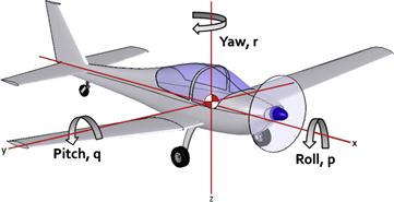
Consider the airplane in Figure 11-1. A conventional stability coordinate-system consisting of x-, y-, and z-axes have been superimposed on the figure. It should be mentioned that in stability and control theory the positive direction of the z-axis always points down, rather than up. The rotation about the x-axis is called roll, the rotation about the y-axis is called pitch, and the rotation about the z-axis is called yaw. Using the right-hand rule of rotation, a positive roll angle is one in which the right wing moves down and the left one up. Similarly, a positive pitch angle is nose-up and negative is nose pitched down. A positive yaw angle is one that moves the nose to the right and negative to the left. These positive rotations are indicated in Figure 11-1. A positive yaw angle is one which would rotate the nose to the right. A positive rudder deflection will generate a positive side force (in the direction of positive y). This means the rudder trailing edge will deflect to the left and a negative (nose left) yawing moment will be generated. A positive elevator deflection (trailing edge down) will produce an increase in lift and pitch the nose down. It is important to keep these conventions in mind for the discussion that follows.
It is important to realize that pitch- and yaw-control can be achieved by other means than just using an elevator and a rudder. For instance, many military fighters combine ailerons and elevator in an all-movable control surface that is located behind the wing, called an elevon. Flying wings often combine the rudder and aileron in a clamshell like control surface on the outboard wing. During flight the upper clamshell is deflected a few degrees trailing edge up (TEU), and the lower one trailing edge down (TED). This generates drag at the wing tips that creates directional stability (this is evident from pictures of the B-2 Spirit Bomber). Such devices are beyond the current discussion. Here we will only consider the more conventional shape, which can be extended to canards and V-tails, although care must be exercised when considering those.
Before any stability and control analysis can begin, the designer must select the type of tail configuration. In other words, will the airplane feature a conventional tail, or T-tail, or other kind of a tail design? Refer to Section 11.3, On the pros and cons of tail configurations, for a discussion on the different kinds of tail surfaces. An imperative element of that decision involves determining how far from the center of gravity (or any other datum point) the tail surfaces should be placed and how large their lifting areas should be. Initial sizing schemes are introduced in this section. The reader should be mindful that ultimately, dynamic stability and handling of the aircraft (spin recovery) will be the final arbiters, but one must begin somewhere and the methods presented herein generally yield a good initial geometry. However, ultimately the aircraft designer should perform dynamic stability analysis. It turns out that an aircraft may be statically stable, but dynamically unstable. A proper dynamic stability analysis will reveal shortcomings and enable the designer to adjust the size or location of the HT and VT (among some other geometric features) such that the aircraft is dynamically stable as well.
11.1.1 The Content of this Chapter
• Section 11.2 presents a general discussion of static stability and control. In addition to defining fundamental stability concepts, it discusses trends in longitudinal and lateral/directional stability derivatives.
• Section 11.3 presents a general discussion of the pros and cons of different tail configurations.
• Section 11.4 defines general horizontal and vertical tail geometry formulation.
• Section 11.5 presents three methods to tailor the tail arm and the vertical tail surface based on the minimum wetted area of a fuselage that has the shape of a frustum. The three methods use the horizontal tail volume, the vertical tail volume, and a combination of the two.
11.1.2 The Process of Tail Sizing
The concept tail sizing refers to the process required to determine the size, shape, and three-dimensional positioning of the stabilizing surfaces. The process of defining the horizontal and vertical tail geometry is accomplished in the following steps:
Step 1: Determine which of the tail configurations in Section 11.3, On the pros and cons of tail configurations, suit the project. Ensure there is a deep and thorough (possibly non-mathematical) evaluation of possible pros and cons, in accordance with the discussion in this chapter, realizing that there may be additional benefits and flaws of each design, not mentioned here. Additionally, there may be other configurations that should be considered besides those presented here. Aesthetics should be seriously considered in this design step. All of the tail configurations presented here will work and have been used on actual aircraft, albeit in different capacities. The primary difference is in the cost of implementation, such as weight, mechanical complexity, and efficiency, to name a few. Unless there is a specific reason for choosing one tail configuration over the others, it will be very helpful to the decision process to draw the proposed vehicle with different tails to help with the tail options, as shown in the examples of Section 11.5, Initial tail sizing methods.
Step 2: Estimate the geometry based on historical data, such as shown in this chapter. This involves estimating the appropriate horizontal and vertical tail volume per Section 11.4.2, Horizontal and vertical tail volumes, and uses these to perform an initial tailoring of the stabilizing surfaces. It must be made clear that this is only an initial estimate based on historical trends. The geometry and characteristics of the airplane, such as the power plant and handling characteristics (both treated elsewhere), will ultimately dictate modification to this initial estimate and this is discussed in Step 3.
Step 3: Once the airplane takes shape, a far more sophisticated resizing, or at least a revision, of the geometry obtained in Step 2 must take place. Such reshaping will depend on a number of factors that do not strictly belong in this chapter. The following bullets constitute design guidelines that all new aircraft should be capable of demonstrating:
• The HT must be capable of trimming the airplane at low airspeeds at a forward CG location. This means airspeed at least as low as 1.2 VS in the landing configuration.
• The HT must be capable of trimming the airplane at high airspeeds at an aft CG location. This means the pilot should be able to trim the aircraft for cruise let-down, i.e. to begin and maintain descent at airspeed as high as cruising speed plus 5 to 10 KTAS.
• The HT and VT must be of a low AR to reduce the risk of tail stall and yet be suitably large AR to make the stabilizing surfaces responsive to AOA or AOY changes. Typically this means that the AR of the HT should be 3 < ARHT < 5 and the VT should be 0.9 < ARVT < 2.
• The VT must provide means to prevent rudder locking. This usually means the addition of a dorsal fin (see Section 11.2.11, The dorsal fin).
• The HT and VT control surfaces must provide enough authority to allow the airplane to be controlled during demanding maneuvers such as balked landing and crosswind landing without excessive control surface deflections.
• The HT must allow the airplane to be stalled. This is imperative because the stalling speed (say +1 knot) is truly the slowest speed the airplane is capable of. If the airplane cannot stall because of limited elevator authority, its minimum speed will be higher than the stalling speed and this can result in higher approach speeds, demand longer runways, and even compromise the certifiability of the aircraft. This may happen if the minimum speed is higher than the regulatory limits (i.e. 61 KCAS for 14 CFR Part 23, or 45 KCAS for LSA).
• The HT and VT must result in stability derivatives such as Cma, Cmde, Cmq, Cyb, Cnb, Cndr, Cnr, and others that ensure the airplane is naturally statically and dynamically stable. All 14 CFR Part 23 aircraft are required to be statically stable and demonstrate stable longitudinal short period and lateral directional oscillation (also known as Dutch roll) modes. However, the designer should strive to make the remaining dynamic modes convergent. Strictly speaking, GA aircraft do not need fly-by-wire control systems because by law they have to be stable. This, however, does not preclude the development of such systems for GA aircraft as these may offer supplemental benefits.
• The HT and VT should not have detrimental impact on the non-linear behavior of the above stability derivatives at high AOAs and AOYs. For instance, the derivatives should not acquire values that render the airplane unrecoverable in spins or deep-stall.
• The HT and VT must be designed for minimum structural weight, with the designer being cognizant of the manufacturability and aeroelastic consequences of a particular design.
• The control system should be simple and reliable and it should not require excessive control surface deflection to maneuver the airplane, even in demanding maneuvers. Large control surface deflection will cause the surface to stall, sharply lowering the control authority.
• If the control system is manual, it should not require excessive control forces to deflect the surfaces throughout the operating envelope of the aircraft. Consult 14 CFR Part 23.155, Elevator control force in maneuvers and 23.397, Limit control forces and torques, regarding regulatory limits.
• The designer must be cognizant of other operational limitations. For instance, excessive length of the tail arm may interfere with T-O rotation, subject the structure to high stresses, and lower the flutter speed of the airplane. Excessively short tail arms will require high deflection angles of control surfaces and may result in poor handling characteristics due to unacceptably low pitch damping.
Many of the above bullets are not treated directly in this section. Among those are the evaluation of dynamic stability and compliance with the design checklist of Section 23.3, Preliminary aircraft design checklist. At any rate, provided the designer does not violate other requirements, drag should always be minimized. Sections 11.4 and 11.5 develop a few techniques intended as a “first stab” tail sizing methods that minimize the wetted area of the empennage in order to reduce skin friction drag.
11.2 Fundamentals of Static Stability and Control
The design of the tail is essential to the safe operation of the airplane. The design is highly dependent on the scientific discipline called stability and control theory. In this context, the science of mechanics is usually broken into two fields: statics and dynamics. Statics considers the equilibrium of matter for which linear and angular acceleration is zero, while dynamics studies the equilibrium of matter that undergoes linear and angular accelerations. Aircraft stability and control is a field within mechanics that applies specifically to vehicles subject to six degrees of freedom motion (three linear and three rotational).
The analysis of the total stability of an airplane is performed by considering the contribution of a number of components. Thus, there is a contribution due to the wings, HT, fuselage, landing gear, and power plant. There can be a further breakdown based on specific components – for instance, the contribution of the wing is broken down into that of the main wing element, flap, leading edge devices, and so forth. The magnitude of these is then summed along and about the three axes, which indicates the instantaneous stability and motion of the aircraft. An airplane can maintain steady unaccelerated flight only when the sum of all forces and moments about its CG vanishes.
Static and dynamic stability analyses revolve around developing the equations of motion, evaluating the component contributions, and using these to evaluate a number of static and dynamic stability characteristics. The standard stability coordinate system is defined so the x-axis points toward the nose, the y-axis points to the right wingtip, and the z-axis points downward. Positive rotations are defined according to the right-hand rule.
11.2.1 Fundamentals of Static Longitudinal Stability
Requirements for Static Longitudinal Stability
Consider the airplane in Figure 11-2. The image to the left shows it at a high AOA and the right one at a low AOA. The figure helps build an understanding of what is meant by longitudinal stability. In the left image, the horizontal tail (HT) generates a lift force, LHT, which points upward and, thus, tends to reduce the AOA by lowering the nose. Using the standard stability coordinate system the resulting moment has a negative magnitude. This means that grabbing around the y-axis with the right hand to generate this nose-down rotation requires the thumb to point in the negative y-direction. To pitch the nose up requires the thumb to point in the positive y-direction.

FIGURE 11-2 The generation of longitudinal stability. The left image has α > 0 and M < 0 (the moment due to LHT tends to pitch the nose down). The right image has α < 0 and M > 0 (the moment due to LHT tends to pitch the nose up). This airplane is statically stable.
The right image of Figure 11-2 shows the opposite. Due to the low AOA, the HT is generating lift in the downward direction causing a tendency to increase the AOA. This requires the moment to have a positive value. This means that somewhere between the two extremes is an AOA for which there is no tendency for the HT to increase or decrease the AOA. This is the trim AOA. An airplane whose stabilizing surface (here the HT) generates enough lift force to force the aircraft to a specific trim AOA is called a stable aircraft.
These two conditions in Figure 11-2 have been plotted in Figure 11-3. The conditions consist of α > 0 and M < 0 in the left image and α < 0 and M > 0 in the right image. The graph shows clearly that in order for the aircraft to be stable, the pitching moment curve must necessarily have a negative slope. This slope is denoted by the symbol Cmα. Additionally, in order to be able to trim the airplane at an AOA that generates positive lift, the intersection to the y-axis (Cm-axis), denoted by Cm0, must be larger than zero. Mathematically, this is written as follows:

FIGURE 11-3 The pitching moment curve must have a negative slope for the airplane to be stable and intersect the y-axis (Cm-axis) at a positive value (Cmo) in order to be trimmable at a positive AOA (necessary condition to generate lift that opposes weight).
If these conditions are satisfied, then there exists an AOA > 0 for which the Cm is equal to zero. The importance of AOA > 0 is that the vehicle can generate lift in the opposite direction of the weight and simultaneously be statically stable – a necessary condition for flying in the absence of stability augmentation systems (SAS). As stated earlier, the former condition is the slope of the pitching moment curve, and is short-hand for:
![]() (11-3)
(11-3)
Note that the subscripts for the moment coefficients differ from those of the force coefficients, where capitalization is used to distinguish between two- and three-dimensional force coefficients. Here, the lowercase subscript of Cm can refer to the pitching moment of both a two-dimensional geometry, such as an airfoil, and a three-dimensional geometry, such as a wing. The distinction must be made by context. While it can be confusing, this is done by convention, as the purpose here is not to introduce a new format, but useful formulation. Thus, Cm can refer to the pitching moment of the airfoil or the airplane, separable by context only.
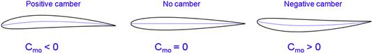
The condition of trimmability for an airfoil can be achieved by selecting the proper camber (see Figure 11-4). The positive camber has a negative Cmo (see Example 11-1), while the opposite is true for one that has a negative camber. In the case of airplanes, a positive Cmo is created by the addition of a stabilizing surface like a HT and by equipping it with an elevator. The elevator allows the moment curve to be moved up or down at will.
To understand why these conditions are necessary consider again Figure 11-3. The solid and dashed lines intersect the horizontal axis approximately at the αtrim = 7.5°. Focusing on the solid line first, consider the aircraft being perturbed from αtrim to, say, 5°. This implies the nose is lower than before and results in a nose-up tendency that will bring the airplane back to αtrim. Similarly, should the perturbation result in a slightly higher AOA, say 10°, the opposite happens and this brings the nose back down to αtrim. Alternatively, if the airplane is statically unstable, as represented by the dashed line, a perturbation that lowers the nose will be accompanied by a tendency to reduce the AOA further. A perturbation resulting in a higher AOA will similarly result in a tendency to increase it further.
EXAMPLE 11-1
Determine the pitching moment curve for the NACA 4412 airfoil in Figure 11-5, if its lift and pitching moment coefficients about the quarter chord are given by the following cubic approximations:
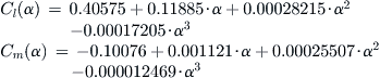
The weight, W, is placed at a distance h from the leading edge. Note that these approximations are shown in the left graph of Figure 11-6. Plot the resulting Cm curve of the airfoil for the following CG locations; h = 0, 0.1, 0.25, and 0.3.
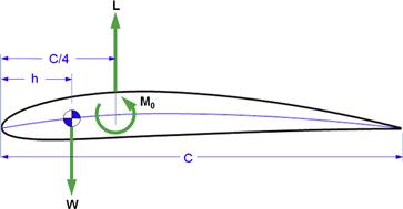
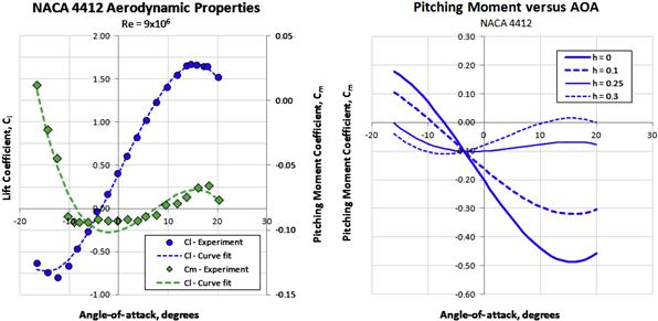
FIGURE 11-6 Experimental and curvefit lift and pitching moment coefficients for the NACA 4412 airfoil (left). Resulting pitching moment curves for the four positions of the CG (right).
Solution
First we note the lift of the airfoil is given by:
![]()
Similarly, the moment is given by:
![]()
where q is the dynamic pressure and C is the chord length. The sum of the moments about the CG (assuming clockwise rotation about the CG is positive) is therefore:
![]()
![]()
Convert to coefficient form by dividing through by qC:
![]()
Insert the cubic splines:
![]()
The resulting plot is shown in the right graph of Figure 11-6. It can be seen that when the weight is at the leading edge (h = 0) the airfoil has the greatest stability of the positions plotted (steepest negative slope). When the weight is at or behind the quarter chord (h = 0.25 and 0.3), the airfoil is neutrally stable or unstable, respectively.
Forces and Moments for Longitudinal Equilibrium
The longitudinal equilibrium requires lift to be equal to weight, drag to be equal to thrust, and pitching moment to be equal to zero. Therefore, the following must hold for longitudinal flight conditions:
Common Expressions for the Aerodynamic Coefficients
In the formulation that follows, the lift, drag, and moment for the entire aircraft are expressed in terms of coefficients that are linear combinations of various contributions. Note that the moment is always taken about the CG (refer to the variable list at the end of the section for the descriptions):
![]() (11-7)
(11-7)
Similarly, the lift coefficient of the tail is given by:
![]() (11-8)
(11-8)
The drag coefficient can be represented as follows:
![]() (11-9)
(11-9)
The pitching moment coefficient can be represented as shown below:
![]() (11-10)
(11-10)
11.2.2 Modeling the Pitching Moment for a Simple Wing-HT System
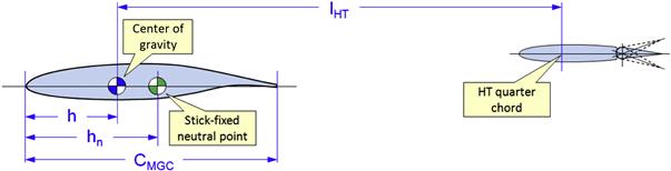
The solid line in Figure 11-3 is the pitching moment curve and is denoted by Cm. It is a function of the AOA and the location of the center of gravity. Consider Figure 11-7, which shows a simple three-dimensional system consisting of a wing and a HT. Shown are two airfoils that represent the mean geometric chord (MGC) of the wing and the HT. Furthermore, it positions the center of gravity (CG) and the stick-fixed neutral point (to be defined later), denoting the former using the term h and the latter hn. It is given by the follow expression:
![]() (11-11)
(11-11)
where
In stability and control theory, the quantity (h − hn)/CMGC is termed Static Margin. It is of utmost importance in the discussion that follows. It can be seen that if the location of the CG moves behind the neutral point, the quantity (h − hn) of Equation (11-11) will acquire a positive value. This means the airplane is unstable – at high AOAs, it will tend to increase its AOA further rather than reducing it and the opposite at low AOAs. This renders the aircraft uncontrollable for human pilots, although it can be controlled by a computer-controlled flight control system (fly-by-wire or fly-by-light). GA aircraft must be designed so they are naturally statically and dynamically stable, although the authorities have proven flexible in the certification of airplanes whose phugoid and spiral stability modes are divergent.
11.2.3 Horizontal Tail Downwash Angle
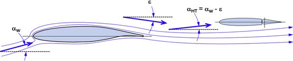
If the wing is placed ahead of the horizontal tail (as is common for most airplanes) it will be subject to downwash that changes the AOA on the tail. For instance, consider the main wing at an AOA of 10°. At first glance, one might assume the horizontal tail is also at an AOA of 10°, but this is not the case. The downwash from the main wing will reduce the AOA on the HT, so it might only be 5°. Clearly this will affect the stability of the airplane and, thus, must be accounted for.
Downwash per the Momentum Theory
The momentum theory represents the simplest method to predict the downwash behind the wing. Its primary shortcoming is it assumes an elliptical planform and returns an average value whereas in real flow the magnitude varies with position in space. Its primary advantage is ease of estimation. Its results are generally acceptable for conceptual and preliminary design; however, using the method to position the height of the HT with respect to the wing is not reliable. The downwash is expressed using the following linear relation:
![]() (11-12)
(11-12)
where ε0 is the residual downwash (when α = 0) which is only present if the wing features cambered airfoils. The derivative dε/dα indicates the change in downwash with AOA. In the absence of more sophisticated analysis, the downwash can be estimated using the momentum theorem of Section 8.1.8, The generation of lift. This allows the downwash angle to be presented in terms of the CLα of the wing per Equation (8-22), repeated below for convenience:
![]() (8-21)
(8-21)
where CLW is the lift coefficient of the wing and not the entire airplane, but the downwash is caused by the wing primarily. The units for the angle are radians. Once the downwash angle is known, it is easy to determine the AOA on the horizontal tail, using the schematic of Figure 11-8.
A more common way of presenting the downwash angle is to write:
![]() (11-13)
(11-13)
where, similarly, CLαW is the lift curve slope of the wing. Therefore, we can define the residual and AOA-dependent downwash as follows:
![]() (11-14)
(11-14)
It is evident from the derivation of the above expressions that they represent the average for the entire column of air being deflected downward to generate lift. In real flow, the size and position of the HT in space will cause the downwash angle to vary along its span. Inserting Equation (11-14) into (11-13) yields:
![]() (11-15)
(11-15)
However, once an angle-of-incidence (AOI) is introduced to the wing and HT, things get a bit more complicated (see Figure 11-9). Note that a positive iW and negative iHT are shown as most aircraft feature that geometry. Increasing the wing AOI is akin to increasing the overall AOA on the wing. When adding iHT to the sum (as shown), it will reduce the AOA on the HT. Therefore, the AOA of the HT can be summarized as follows:
![]() (11-16)
(11-16)
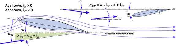
FIGURE 11-9 A schematic showing how introducing an AOI of the wing and HT the downwash angle, ε, affects the AOA on the horizontal tail.
It is convenient to define the AOA of the wing-body combination as shown in Figure 11-9 and write Equation (11-16) as follows:
![]() (11-17)
(11-17)
11.2.4 Historical Values of Cmα
As stated earlier, the purpose of the HT and VT is to make the airplane controllable and provide it with acceptable static stability. The term “acceptable static stability” is somewhat nebulous and depends on the class of airplanes being considered. It refers to the magnitude of the slope of the pitch stability, Cmα. Thus, transport aircraft usually have “high” pitch stability, which is reflected in a low value of Cmα, often in the −1.2 to −1.7 per radian range. GA aircraft are typically in the −0.6 to −1.0 per radian range. On the other hand, the modern fighter aircraft is purposely unstable (Cmα > 0).
During the design of the aircraft it is important to know what longitudinal stability derivatives to aim for. As usual, the history of aviation presents us with a large number of candidate values. Table 11-1 lists a number of longitudinal stability derivatives, gathered from Refs 1, 2, 3, and 4, and the author’s personal notes. A selection of the airplanes is shown plotted in Figure 11-10.
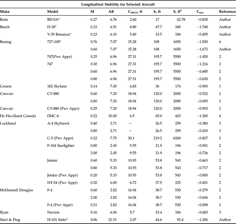
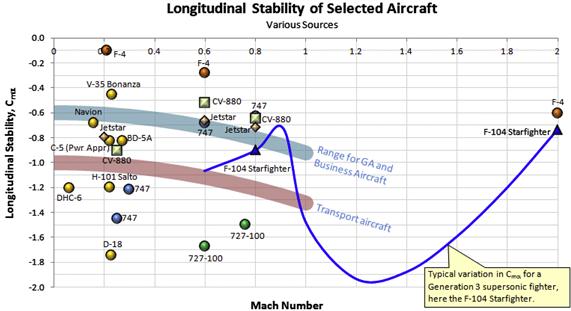
A high level of stability is a good quality in a transport-class aircraft, as the pilot (or the autopilot) will not have to work hard to maintain steady level flight. This is also a requirement by 14 CFR Part 23.173 (see introduction to this section) for GA aircraft and 25.173 for commercial aircraft. The primary drawback is reduced maneuverability (the rate at which the aircraft’s orientation can be changed), but this is a secondary priority for transport aircraft – they only have to be maneuverable enough to allow for safe flying. Fighter aircraft, on the other hand, represent the other extreme. A fighter must be highly maneuverable as this, in addition to its energy level, largely dictates whether it can beat an opponent in a dogfight. Such aircraft have very high wing-loading and a high moment of inertia. If made too stable, the resulting aircraft would be unacceptably sluggish. The solution is a reduction in the static stability as this increases the maneuverability. In fact, the modern fighter is longitudinally unstable for this reason. The drawback is that it requires a computer-managed control system to control such an aircraft (fly-by-wire or the more modern fly-by-light). One important consequence of supersonic flight is that the center of lift moves aft, and this increases static stability. Thus, the modern fighter aircraft is longitudinally unstable while subsonic, but stable when supersonic. The static stability of GA aircraft fits snugly between these two extremes.
Note that although this book focuses on GA aircraft, it is still of interest to see how the derivatives are affected by high Mach numbers. For this reason, high speed values are included. It is important to realize that the Cmα is not truly a constant. It changes with Mach number because of compressibility effects, as well as when the airplane’s configuration changes as a result of retracting landing gear and flaps. Compressibility effects are shown for the F-104 Starfighter, a third-generation fighter, as the solid line in Figure 11-10, which explains why its stability derivative, Cmα, is less than zero over its Mach range. Marginally stable and unstable fighters emerged first with fourth-generation fighter aircraft. Also, note the range of stability of the F-4 Phantom fighter (also third-generation) which is marginal at M = 0.2 (landing configuration), but becomes noticeably stable at M = 2. Also notice how the Mach number changes the longitudinal stability of commercial jetliners, like the Boeing 727, 747, and the Convair CV-880.
11.2.5 Longitudinal Equilibrium for Any Configuration
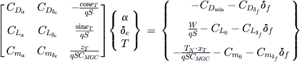
One of the most important benefits of the longitudinal stability equations (see Equations (11-4) through (11-6)) is their use for determining the static stability. The following formulation is used to determine the AOA (α), elevator deflection (δe), and thrust (T) required for steady level flight. It is applicable to almost any configuration, as long as the stability derivatives are determined correctly. Converting these equations to a coefficient form yields:
![]() (11-18)
(11-18)
![]() (11-19)
(11-19)
![]() (11-20)
(11-20)
where εT is the thrust force angle. The coefficients are the sums of the coefficients determined in the previous section. For instance, Cmα is the sum of the contribution of the wing, HT, fuselage, landing gear, etc. The same holds for the other coefficients. Therefore, it is first necessary to rearrange the above equations:
![]() (11-21)
(11-21)
![]() (11-22)
(11-22)
The moment equation poses a bit of a problem when dealing with propeller normal force, reflected in the coefficient ![]() . The propeller normal force depends on thrust, but it is one of the unknowns. Therefore, the moment portion would have to be solved iteratively, which is not always convenient. The usual remedy is to omit thrust from the solution and solve only for α and δe. However, here, we also want to estimate thrust requirements as this gives important clues about the capability of the aircraft, such as, does it have enough power or thrust to sustain level flight at the selected airspeed? The moment equation is written as shown in Equation (11-23):
. The propeller normal force depends on thrust, but it is one of the unknowns. Therefore, the moment portion would have to be solved iteratively, which is not always convenient. The usual remedy is to omit thrust from the solution and solve only for α and δe. However, here, we also want to estimate thrust requirements as this gives important clues about the capability of the aircraft, such as, does it have enough power or thrust to sustain level flight at the selected airspeed? The moment equation is written as shown in Equation (11-23):
The workaround for the normal force problem is to treat it as a constant and calculate an average around an expected thrust value. This will reduce the error in the solution. The other option, as stated above, is to solve for the thrust and use that to calculate the normal force. Using that value the thrust is calculated again and used to get a new value of the normal force, and so on, until both approach a fixed value. In either case, Equation (11-23) can be written as shown in Equation (11-24):
![]() (11-24)
(11-24)
The equations can now be rearranged in the following matrix form of Equation (11-25):
 (11-25)
When solved, Equation (11-25) yields the AOA, elevator deflection, and thrust required for a longitudinally stable flight at a given airspeed and atmospheric conditions. The solution can be implemented using a simple method such as the 3 × 3 Cramer’s Rule. Once implemented, the formulation can be used to estimate suitable elevator deflection range (by varying the CG location) and power requirements at various conditions, including high altitudes and with flaps (or landing gear) deployed.
Note that typical values of the derivatives for small GA aircraft fall within the following limits (note that all the derivatives are in terms of radians; note that all angles, α, δe, and δf are in radians):
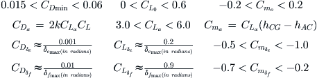
Typical δemax is 20°–25° (0.349 – 0.436 radians) and δfmax is 30°–45° (0.524 – 0.785 radians). These are only intended to give “ballpark” numbers and are not a substitute for analysis. The derivatives of your airplane may deviated greatly from these. Also see Appendix C1, Design of Conventional Aircraft for additional tail sizing tools.
EXAMPLE 11-2
Determine the α, δe, and T required for a stable level flight with flaps retracted at S-L and (a) 180 KCAS (q = 109.8 lbf/ft2) and (b) 75 KCAS (q = 19.06 lbf/ft2). The aircraft weight amounts to 3400 lbf, S = 144.9 ft2, CMGC = 3.78 ft, xT = 13.06 ft, zT = −0.5 ft, ε = 0°, k = 0.04207 and the pertinent coefficients are given by:
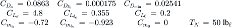
Note that all the stability derivatives are in terms of radians. If we assume propeller efficiency, ηp, of 0.85 for the high-speed case and 0.60 for the low-speed one, how much engine power is required to achieve this? Use Equation (14-38).
Solution
(a) Begin by populating the matrices of Equation (11-25):
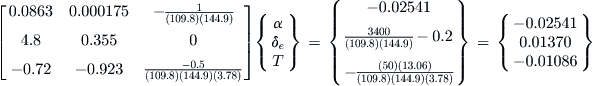
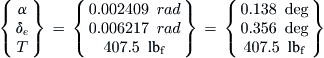
Then, solve for the three arguments α, δe, and T, using any matrix method. Here the solution yields:
The power requirements are thus:
![]()
(b) Proceed in a similar manner, except note that ![]() changes to 0.4973. The results are:
changes to 0.4973. The results are:
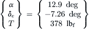
The power requirements are thus 145 BHP or about 47% power. In reality this power is underestimated as it is based on the simplified drag model (see Chapter 15, Aircraft drag analysis), which under-predicts the drag at high lift coefficients.
11.2.6 The Stick-fixed and Stick-free Neutral Points
As the CG of an aircraft is moved from a far forward to a far aft position (e.g. by moving useful load around), its longitudinal stability derivative, Cmα, is modified greatly, from a large negative number to a large positive number (relatively speaking). This is reflected in Figure 11-3, which shows Cm(α) with both a positive and negative slope. As has already been discussed, the positive slope means the vehicle is statically unstable. By law, GA aircraft must be stable. For this reason, it is vital to be able to determine the CG location at which the slope becomes zero. This important point is called the neutral point.
There are two types of neutral points: stick-fixed and stick-free. The former refers to the stability with the elevator fixed in its neutral position (0° deflection angle), while the latter refers to the elevator being free to move. This distinction is of considerable importance, because at a given AOA (assuming α > 0), a conventional elevator tends to float trailing edge up (as if to “help” the airplane getting to an even larger AOA). Therefore, the airplane is less stable than if the elevator is fixed. It should be evident that for typical aircraft, the stick-free neutral point should be expected to be farther forward than the stick-fixed one.
An important note should be made here regarding the stick-free neutral point. It is indeed possible for it to be aft of the stick-fixed neutral point. This depends on the magnitude of hinge moments due to deflection and AOA on the HT. However, during the conceptual design phase, a forward-lying stick-free neutral point is more critical as it narrows the CG envelope for conventional aircraft. And therein lies the problem with its determination; it depends on the elevator hinge moment. This, in turn, depends on the geometry of the horizontal tail, the size of the elevator, hinge line location, airfoil, the presence and geometry of a control horn, deflection of a trim tab, and other factors (see Section 23.2.1, Introduction to control surface hinge moments). Such details are simply not known during the conceptual design phase and this calls for some assumptions to be made to allow the HT to be sized.
On the other hand, the stick-fixed neutral point is less hard to determine, although it is by no means simple. The following method allows the first stab at the stick-fixed neutral point to be made. Then, the stick-free neutral point may be assumed to lie approximately 5% MGC ahead of the stick-fixed, allowing a preliminary aft CG limit to be established. This will have to be revisited and estimated more accurately before the first flight of the prototype, when the geometry of the HT is known in detail. For more information on the generation of the CG-envelope refer to Section 6.6.12, Creating the CG envelope.
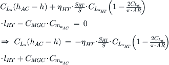
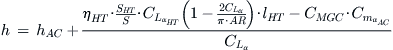
The stick-fixed neutral point can be determined using the following expression, where the physical characteristics refer to those in Figure 11-11:
![]() (11-26)
(11-26)
FIGURE 11-11 Wing-HT system used to derive Equation (11-26).
where
hn = physical location of the CG at which Cmα = 0; i.e. the stick-fixed neutral point
hAC = physical location of the aerodynamic center
ηHT = tail efficiency (see discussion in the derivation)
![]() = longitudinal stability contribution of components other than the wing
= longitudinal stability contribution of components other than the wing
Note that the term ![]() refers to the stabilizing effects of components such as the fuselage, nacelles, landing gear, the wing itself, and so on, as a function of the AOA. If the sum acts to rotate the LE down, then
refers to the stabilizing effects of components such as the fuselage, nacelles, landing gear, the wing itself, and so on, as a function of the AOA. If the sum acts to rotate the LE down, then ![]() (has a negative sign and is stabilizing). If it acts to rotate LE up, then
(has a negative sign and is stabilizing). If it acts to rotate LE up, then ![]() (has a positive sign and is destabilizing). The sign ultimately depends on the aircraft configuration. Note that the destabilizing effects of fuselages and nacelles can be estimated using the so-called Munk-Multhopp method, which is presented in Appendix C1.6, Additional Tools for Tail Sizing.
(has a positive sign and is destabilizing). The sign ultimately depends on the aircraft configuration. Note that the destabilizing effects of fuselages and nacelles can be estimated using the so-called Munk-Multhopp method, which is presented in Appendix C1.6, Additional Tools for Tail Sizing.
Derivation of Equation (11-26)
It is imperative to keep the orientation of the MAC in mind in the following derivation. First, determine the sum of moments about the CG. For static stability, this must equal zero:
![]() (i)
(i)
Note that the sign for MAC here is “+”. Therefore, if MAC is stabilizing (![]() ) we will get +(−|MAC|) = −MAC, where |.| stands for the absolute value. Insert the definitions of
) we will get +(−|MAC|) = −MAC, where |.| stands for the absolute value. Insert the definitions of ![]() , the lift of the HT, given by
, the lift of the HT, given by ![]() , and
, and ![]() and simplify. Also note that the pitching moment coefficient about the aerodynamic center is given by:
and simplify. Also note that the pitching moment coefficient about the aerodynamic center is given by: ![]() . This of course implies its dependency on the attitude (or AOA) of the airplane.
. This of course implies its dependency on the attitude (or AOA) of the airplane.
The term ![]() is the tail efficiency factor. It ranges from 0.8 to 1.2, where numbers larger than 1 represents situations where a part of the HT is inside a propwash. Note that the sign for MAC is now “−”. Therefore, if MAC is stabilizing (
is the tail efficiency factor. It ranges from 0.8 to 1.2, where numbers larger than 1 represents situations where a part of the HT is inside a propwash. Note that the sign for MAC is now “−”. Therefore, if MAC is stabilizing (![]() ) we will get –(–|
) we will get –(–|![]() |) = +
|) = +![]() .
.
Next, insert the definitions for ![]() and
and ![]() and divide through by q·S, as shown below:
and divide through by q·S, as shown below:
![]()
Next, assume the HT features a symmetrical airfoil, i.e. ![]() :
:
![]() (ii)
(ii)
The AOA of the HT is affected by downwash from the wing upstream and can be approximated using the following expression (here assuming no angle-of-incidence). Note that accounting for the AOI is not necessary, as it will only affect the trim point (i.e. shift the Cm curve up or down) and not modify the slope of Cmα:
![]()
A simple approximation for the rate of change of downwash with AOA is given by Equation (8-22) and is only valid for elliptical wings. However, it will give a reasonable prediction for other wing styles and, since we are eager to find out the approximate location of our stick-fixed neutral point, we employ it: ![]() . Inserting this into Equation (ii) yields:
. Inserting this into Equation (ii) yields:
Now, let ![]() and recall that
and recall that ![]() , simplify by gathering like terms:
, simplify by gathering like terms:
To determine the neutral point, the term inside the bracket must equal zero, i.e.:
![]() (iii)
(iii)
This depends primarily on the location of the CG, denoted by h. Rearranging Equation (iii) in terms of h yields:
This allows the location of the stick-fixed neutral point to be determined from:
Since this point is typically denoted by hn, we replace h by this symbol below. It is more convenient to be able to express the dimensions h and hAC in terms of the fraction of chord length at the MGC, here denoted by CMGC. For this reason we divide through by CMGC:

Finally, define ![]() as the horizontal tail volume and insert to obtain Equation (11-26).
as the horizontal tail volume and insert to obtain Equation (11-26).
QED
EXAMPLE 11-3
Determine the stick-fixed neutral point of the Cirrus SR22, using the following data, in part using geometry obtained from Figure 16-15 and Table 16-6, and in part by applying the methods of Chapter 9, The anatomy of the wing, to both the wing and HT geometry. First do this by ignoring the presence of the fuselage and, then, by assuming the token value given below for ![]() .
.
11.2.7 Fundamentals of Static Directional and Lateral Stability
Before embarking on the analysis of lateral and directional stability, a few terms must be defined.
Roll or Bank
An airplane is said to be rolling or banking if a line drawn from wingtip to wingtip (assuming a symmetrical airplane) or some other normally horizontal reference line is sloped with respect to the y-z-axis as defined in Figure 11-1. This implies a rotation about its longitudinal axis – the x-axis or the roll-axis. Roll is the primary method used to change heading (direction of flight) and is controlled using the ailerons. The rudder is merely used to “fine tune” the heading change through coordination – in other words prevent skidding or slipping (discussed below).
The reason why the rudder is far less effective in changing heading than the bank maneuver can be explained using mechanics. A heading change results from acceleration in the horizontal plane that changes the original flight direction. To accomplish this rapidly, substantial force is required. The force generated by the VT through the deflection of a rudder is not a force large enough to change the heading fast enough for safe flight – for this a side force obtained using wing lift is required.
Yaw
An airplane is said to be yawed if its centerline is not parallel to the x-z-plane. This implies a rotation about its vertical axis – the z-axis or the yaw-axis. Based on the assumption that most airplanes are designed to be symmetrical about the x-z-plane, this rotation makes it un-symmetrical with respect to the airflow, which inevitably generates a side force and moment about the yaw axis.
Slipping or Sideslip
If the airplane is “yawed out of a turn”, i.e. if the nose points outside of the trajectory of the turn, it is said to be slipping (see Figure 11-12). If banking left, this means the nose points to the right. Effectively, the bank angle of the airplane is steeper than the rate of turn would indicate. Slips primarily happen in two ways: as a consequence of uncoordinated deflection of ailerons and rudder; or the consequence of the intentional application of opposite rudder during a bank to increase drag or align the ground track while landing in a crosswind.

Slip is a trick sometimes used by pilots for altitude or airspeed control because the yaw that results increases the drag of the airplane.
If the airplane is “yawed into a turn”, i.e. if the nose points to the inside of the trajectory of the turn, it is said to be skidding (see Figure 11-12). If banking left, this means the nose points further left than the rate of turn indicates; the bank angle of the airplane is shallower than indicated by the rate of turn. Skids primarily happen in two ways: (1) as a consequence of uncoordinated deflection of ailerons and rudder or (2) the consequence of the intentional and excessive application of pro-bank rudder.
All aircraft certified to 14 CFR Part 23 must be demonstrably laterally and directionally stable per 14 CFR 23.177 Static Directional and Lateral Stability. For this reason, slipping and skidding are pilot-induced maneuvers, as the airplane must be designed to suppress them. However, they may occur because of an airplane operating with asymmetric thrust, such as a multiengine aircraft with one engine inoperable (OEI).
11.2.8 Requirements for Static Directional Stability
Directional stability is the capability of the vehicle to weather vane. Imagine standing behind an actual weather vane with the wind directly in your face. If the vane is rotated so its nose points, say, right (and the tail points left) intuition tells us its tail will generate lift that points to the right, in the positive y-direction (see depiction in Figure 11-13). This, in turn, generates a moment whose tendency is to rotate the nose left and align it (and the tail) with the wind. Since the moment corrects the alignment, it is said to be restoring.
If the above weather vane is yawed nose right, then, using the stability coordinate system (SCS), the angle β < 0°. This means that if looking along the centerline of the vane, the wind would strike the left cheek. The restoring moment is negative because per the right-hand rule, the resulting rotation is analogous to grabbing around the z-axis with the right hand to rotate it with the right thumb pointing upward – in the negative z-direction. The opposite holds true if the weather vane is rotated nose left – a positive moment (thumb pointing down) is then required to bring the nose right to the initial position.
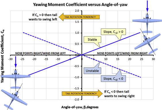
Figure 11-13 shows how this establishes requirements for static directional stability. It turns out that in order for this correcting tendency to be realized, the slope of the yawing moment curve must have a positive slope. Mathematically this is written as follows:
11.2.9 Requirements for Lateral Stability
Next consider lateral stability (see Figure 11-14). It differs from both longitudinal and directional stability in that it requires sideslip (or yaw), and not roll itself, to be corrected (ignoring the application of devices like ailerons). This is the aforementioned dihedral effect. The geometric features of airplanes are such that when flying asymmetrically a restoring rolling as well as directional moments are created. It is the responsibility of the designer to decide how to manipulate the geometry to make these moments restoring or convergent (and not diverging). Dihedral effect has many sources as will become evident shortly.
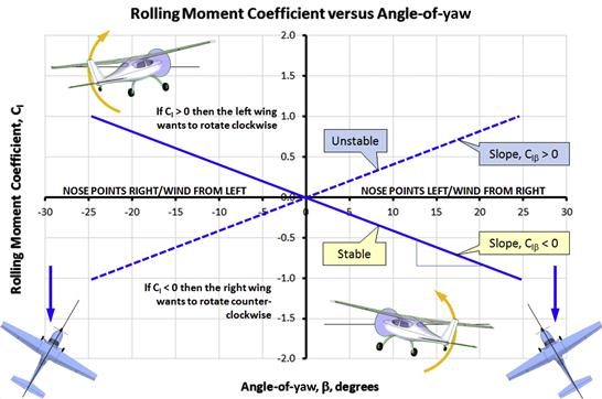
Consider the airplane in the upper left part of Figure 11-14, whose nose points to the right of the wind direction (which is normal to the plane). For now consider only the contribution of the wing to the rolling moment. It can be seen from the top view in the lower left corner that the left wing leads the right one. This causes asymmetric loading on the wing that generates more lift on the left wing than the right one. The difference creates a rolling moment that tends to lift the left wing and bring it back to level. The rolling moment is positive because, according to the right-hand rule, the resulting moment vector points forward (the thumb would point forward) along the positive x-axis. The opposite holds if the nose is yawed to the left so the right wing leads the left one; a negative moment is created. By plotting a line between those two conditions, as is done in Figure 11-14, it can be seen that the rolling moment must have a negative slope in order to be stable. Mathematically:
11.2.10 Historical Values of Cnβ and Clβ
During the design of the aircraft it is important to know what directional and roll stability derivatives to aim for. As usual, the history of aviation presents us with a large number of candidate values. Table 11-2 lists a number of directional and lateral stability derivatives, gathered from References [1, 2, 3, and 4], and the author’s own estimations. A selection of the airplanes are shown plotted in Figure 11-15 and Figure 11-16.

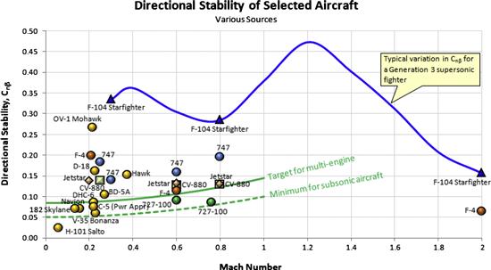
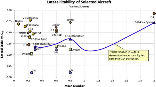
Note that although this book focuses on GA aircraft, it is still of interest to see how the derivatives are affected by high Mach numbers. For this reason, high-speed values are included.
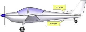
11.2.11 The Dorsal Fin
A dorsal fin is a small surface extension installed at the leading edge of the root of the vertical tail (see Figure 11-17). Its purpose is to add directional stability to the aircraft and that way prevent a serious condition known as rudder-lock. The dorsal fin, or dorsal as it is often referred to, can be as simple as a thin flat plate or as complicated as a curved compound surface stamped aluminum fairing riveted to an existing fin. In any case, its presence causes the leading edge to feature a discontinuity and this is imperative to its functionality. Older aircraft, such as the Douglas DC-4 (see Figure 11-18), DC-6, and many others) have curved dorsal fins, whose leading edges appear continuous, mathematically, and this makes it hard to perceive a specific discontinuity. However, this in no way prevents the formation of a vortex over the vertical tail.
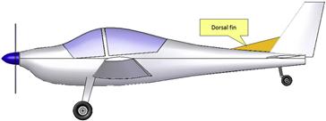
FIGURE 11-17 The dorsal fin is a surface extension between the VT and the fuselage, whose purpose is to improve directional stability at high angles of yaw.
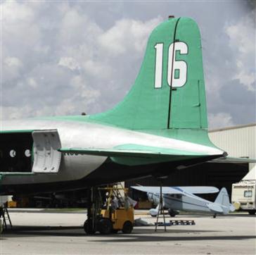
FIGURE 11-18 A dorsal fin on the Douglas DC-4 is typical of aircraft of that era, featuring a mathematically continuous and smooth curved leading edge. (Photo by Phil Rademacher)
The phenomenon of rudder locking is largely caused by insufficient directional stability of the airplane at high AOYs. As the airplane is yawed to a high AOY (for instance in a side-slip maneuver) two things may happen:
(1) If the vertical tail is poorly designed (e.g. features excessively large AR and small area) it may stall. A consequence of this will be a sharp drop in directional stability. The drop may be enough for the restoring moment generated by the vertical tail to be less than the destabilizing moment generated by the fuselage.
(2) The side loading resulting from the yaw will tend to force the rudder to the leeward side (if it is not there already as it may have been used to drive the airplane to this condition in the first place). This reduces the yaw contribution of the vertical tail further. If the hinge moments of the rudder are high, this compounds the problem by making it impossible for the pilot to step on the opposite rudder to recover from the situation. This way, the rudder is effectively “locked,” hence the name.
A classic example of the severity of the rudder-locking problem was recorded on March 18, 1939, when an early production version of the Boeing 307 Stratoliner crashed during an evaluation test flight, killing all 10 people on board [5]. Officials of the Dutch airline KLM had expressed interest in the aircraft and sent a test pilot to evaluate it. The airplane, slated to be delivered to Pan Am, was at 10,000 ft when the KLM pilot shut down two of its engines on the same wing to evaluate its asymmetric thrust characteristics. He brought it to maneuvering speed, where it stalled and entered spin. The rudder locked during the spin, making recovery attempts by its two pilots impossible [6]. It is thought these attempts caused the wing and empennage to separate from the rest of the airplane. Wind tunnel testing after the mishap showed that the original tail on the airplane was too small and rudder area too large. It demonstrated that adding a dorsal would remedy the problem [7].
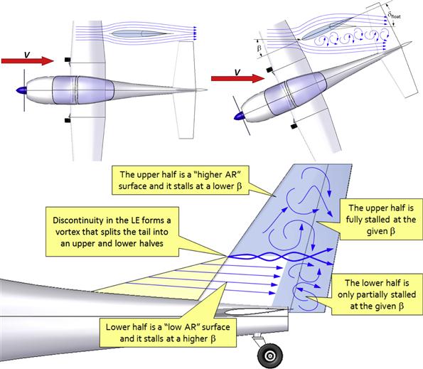
One solution for a rudder lock condition is to mount a dorsal to the fin. This will partition the vertical into two low-aspect-ratio segments. The smaller one will remain unstalled to an even higher yaw angle (because small AR surfaces stall at a higher AOA than high AR surfaces) and this helps maintain sufficient directional stability up to the higher AOY than without it.
Another solution, often featured on aircraft designed in the 1930–1940s, is an H-tail configuration, with small low-aspect-ratio (AR∼1) tail surfaces. Such surfaces stall at very high AOAs, as high as 30°–40°.
In the absence of the dorsal, the entire tail would be stalled. Its presence introduces a discontinuity in the leading edge of the VT, which at non-zero AOY generates a vortex as shown in Figure 11-19. The vortex effectively splits the fin into upper and lower halves. The upper half has a higher AR than the lower one and, thus, stalls at a lower AOY. And that is the important thing. The fact that the lower half is only partially stalled renders the Cnβ greater than if the dorsal was absent. This allows the Cnβ to be maintained to a higher AOY. Not only is the Cnβ increased due to the added area of the dorsal, it also guarantees it stays higher to greater AOY.
The recovery from a rudder lock requires the airspeed to be reduced by a roll or a pull-up maneuver to be performed or so the hinge moment drops to a magnitude that allows the pilot to bring the rudder to neutral with force [7, p. 221].
11.2.12 The Ventral Fin
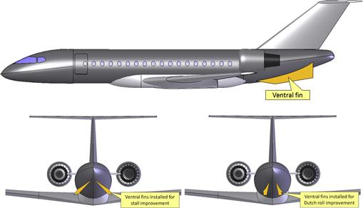
The ventral fin is a lifting surface used for two purposes: to improve stall, or Dutch roll characteristics. Dorsal fins are rarely installed for other purposes, although the author of this book was involved in a project that featured one purely for looks (misguided one might add). The installation of a ventral fin typically means two things: there is insufficient nose pitch-down moment at stall; and there is insufficient Dutch roll damping. It is relatively easy to identify the reason for installation, as ventral fins installed for the former are usually substantially more horizontal than the latter (see Figure 11-20).
Ventral fins generally work as follows. At cruise AOAs the AOA of the ideal ventral fin will be very low. This is necessary as it is essentially an aerodynamic fix for a high AOA condition and, thus, at cruise its drag should be as low as possible. Then, as the pitch angle (AOA) of the airplane increases the ventral becomes gradually more effective and it will begin to contribute to the longitudinal stability. This is depicted in Figure 11-21. The reader should also review Section 11.3.3, T-tail, for further insight.

FIGURE 11-21 A ventral fin installed to prevent deep-stall changes the shape of the pitching moment curve such that a trim point no longer exists in the post-stall region.
The solid curve in Figure 11-21 represents the pitching moment curve for a hypothetical airplane. It can be seen that the nonlinearity in the original aircraft result in a trim point around 32°. If this airplane for some reason reached that AOA, it would not have the elevator authority to recover (note that the graph represents the condition at full elevator aft condition; also refer to Figure 11-33 for further insight). The installation of the ventral will increase the nose pitch-down moment at this condition, effectively deleting the trim point. This would allow the modified aircraft to recover from the condition – it would not be affected by a deep-stall.
The installation of ventral fins must take into account the three-dimensional shape of the flow field around the aft end of the airplane, often rendering the orientation of the ventral fin somewhat “unintuitive.”
11.2.13 Tail Design and Spin Recovery
Spin entry and recovery is of major concern in GA aircraft. Spin is a consequence of asymmetric wing stall that typically results in an inadvertent wing roll to the left or right, initiating a dynamic mode called autorotation. The motion is a rapid vertical descent along a helical path. The autorotation is caused as the lower wing, i.e. the wing on the inside of the yawing motion, has a higher AOA than the higher wing (the outside wing). The difference in AOA results in a difference in wing lift between the two wing halves, such that the outside wing lift is greater and this drives the rotation.
Spin regulations for certified GA aircraft are presented in 14 CFR 23.221, Spinning. The paragraph states that a normal, utility, and aerobatic category aircraft for which spin certification is sought “must be able to recover from a one-turn spin or a three-second spin, whichever takes longer, in not more than one additional turn after initiation of the first control action for recovery, or demonstrate compliance with the optional spin resistant requirements of this section.”
The arrangement of the HT with respect to the VT is of great concern in aircraft design. This is because the wake generated by the HT may “blanket” the rudder, rendering it far less effective than otherwise. Blanketing means that the rudder is largely covered by separated airflow, but this may reduce its effectiveness so it becomes incapable of providing adequate counter-rotational moment during spin. This can cause a serious problem when attempting spin recovery, at times making it altogether impossible. Figure 11-22 shows common HT/VT arrangements and idealized wakes emanating from the HT. Some of the configurations are void of separated flow (e.g. V-tail, T-tail, and H-tail), whereas the conventional configuration is exposed to different levels of blanketing.
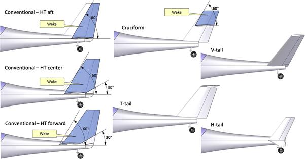
FIGURE 11-22 The blanketing of the rudder during spin is largely dependent on the tail configuration.
It must be said that the flow field around a spinning airplane is very complex and the spin is driven by a difference in the lift generated by the left and right wings. The flow field is further compounded by contributions from the fuselage, so what is said here really represents rules of thumb. It is generally recommended that at least 1/3 of the rudder should remain in undistorted airflow. The figure shows three conventional configurations, of which only the bottom one has that much rudder area in “clean” air. Figure 11-23 shows a possible solution to a spin recovery problem – increase in vertical surface area using dorsal and ventral fins. There is no guarantee such a solution will work, but if it does, it usually affects the aesthetics of the airplane.
11.3 On the Pros and Cons of Tail Configurations
The purpose of this section is to introduce a number of the various tail configurations that have seen use throughout the history of aviation. The selection itself can only be made easier if the designer is aware of the many advantages and disadvantages of each configuration, in terms of aerodynamics; stability and control; structural layout; aeroelasticity; and operational characteristics.
11.3.1 Conventional Tail
The conventional tail is the most common of all tail configurations. Possibly some 80% of aircraft ever built feature this tail configuration, ranging from ultralight aircraft to the world’s largest passenger transport aircraft, the Airbus A380 and Boeing 747. A large number of GA aircraft also feature the tail, such as the Cessna single-engine series aircraft (140, 150, 152, 172, and so on) as well as the latest entries, the all-composite Cirrus SR20, SR22, and Cessna Corvalis high-performance aircraft. The configuration is often a “default” configuration unless some special requirements call for alternative solutions. For the discussion that follows, this configuration is considered the “baseline” configuration (see Figure 11-24).
The advantages of this configuration are many, beginning with it being a safe-and-tried configuration as evidenced by the fact that the majority of airplanes feature it. For single-engine propeller aircraft the configuration takes advantage of the propwash, which gives it a boost during the T-O run. This makes it possible to rotate at a lower airspeed, reducing the ground run (see the discussion about drawbacks below).
The horizontal tail is sometimes positioned so the wing wake at high AOA hits the tail, causing it to oscillate (often violently), providing a natural feedback to the pilot of an imminent stall, and then exiting the wake in the post-stall to allow for ready recovery (although often it remains inside the wake). This phenomenon is illustrated in Figure 11-25. Achieving this reliably and by design (as compared to “luck”) requires a thorough understanding of the flow field behind the wing and calls for wind tunnel testing or computational fluid dynamics (CFD) analysis. It is also possible the tail can be positioned such that as the flaps are deployed, the increased nose pitch-down moment may be cancelled by an increase in downwash on the HT, which provides the necessary nose pitch-up moment. This would result in an aircraft that experiences modest, if any, change in trim settings when the flaps are deployed. However, the phenomenon is airspeed-dependent and, thus, cannot always be taken advantage of.
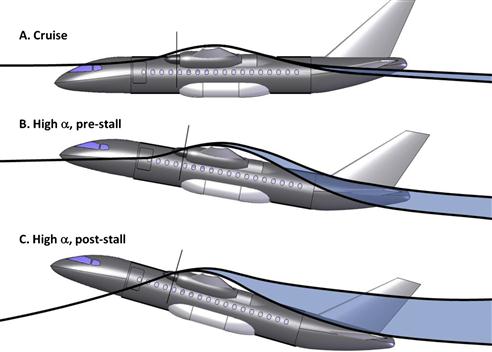
FIGURE 11-25 An aircraft at three different conditions. At cruise (A), the wing wake lies below the HT, but near stall it may strike the HT (B), causing it to oscillate, warning the pilot of an imminent stall. At post-stall (C), the HT may exceed the lower boundary of the wake, although this ultimately depends on the geometry of the airplane.
Another advantage is that the HT and VT are joined in the fuselage, where its girth is still somewhat large and, thus, is still effective in reacting torsional loads. This torsional rigidity also helps resisting empennage flutter.
Figure 11-25 shows an airplane at three specific elevator deflections and AOA. The top figure (A) shows it at a low AOA during cruise. The wing wake lies below the HT and its thickness is relatively small. The center figure (B) shows it at a high AOA, just before stall. The thickness of the wake has grown substantially and now the HT is inside it. The turbulent airflow would cause the tail to oscillate, and the pilot would sense this in the control stick (or yoke) in a mechanical control system, as is the norm for smaller aircraft. However, the pilot might detect structural oscillations even if equipped with a digital control system. The bottom figure (C) shows the aircraft at a post-stall condition, with a fully stalled wake. Depending on its thickness, the HT may or may not reside inside the wake. If inside the wake, the elevator authority is noticeably reduced.
Figure 11-26 shows the Cm versus AOA for the aircraft during the above events (labeled A through C). Point A is trim point for a condition where the elevator deflection might be 3° TED. Point B represents an elevator deflection of 20° TEU and the aircraft is close to stall. Point C represents the aircraft, still with the elevator deflected 20° TEU, at an AOA of 25°, inside the post-stall region. Point D represents the condition of Figure 11-27, deep inside the post-stall region. Some aircraft, for instance the Cirrus SR20 and SR22, are designed to be laterally controllable in this condition, as a part of their Equivalent Level of Safety (ELOS) certification. However, many others are not. Some of those would experience uncontrollable roll tendency to the left or right.
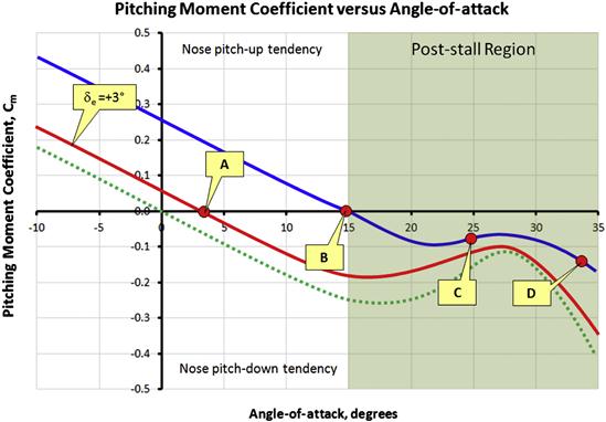
FIGURE 11-26 The conditions for the aircraft in Figure 11-25 and Figure 11-27.
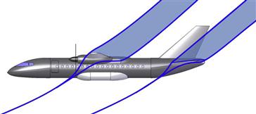
FIGURE 11-27 The same aircraft at a high AOA in a post-stall condition. The shaded areas represent the highly separated wakes emanating from the wing and HT. The HT wake covers a substantial portion of the rudder, reducing the rudder authority. This is Point D in Figure 11-26.
Note that the upper half of the graph is labeled “Nose pitch-up tendency” and the lower half is labeled “Nose pitch-down tendency.” This refers to the corrective tendency displayed by a statically stable airplane. For instance, consider an airplane trimmed at Point A using the center curve. If for some reason it is displaced to a lower AOA (i.e. nose down), it would effectively be moving from the trim point (A) along the curve to some positive value of Cm. This positive Cm would force the nose back up to the AOA at Point A. This would be reversed if it were displaced to a higher AOA (i.e. nose up) – this would generate a tendency to bring the nose back down to Point A.
The primary drawback of the conventional tail is that the wake from the HT may “blanket” the rudder at AOA in the post-stall range (which may easily involve in very high AOAs), although many such aircraft are specifically designed to ensure that adequate rudder area is outside the separated region. Aerobatic aircraft such as the Yakolev Yak-55 and the Extra 300 are examples of this. A blanketed rudder is very undesirable in abused flight conditions such as during a spin (see Figure 11-27) and makes recovery more challenging. The separated flow in the wake reduces the rudder authority substantially and may render the aircraft unrecoverable. However, one should not overlook the fact that a large number of aircraft known for excellent spin recoverability, such as the aforementioned aerobatic aircraft, feature conventional tails. Spin is a very complicated phenomenon and recoverability is affected by a great many features of the airplane besides the blanketing of the rudder. It is only a part of the puzzle. Also, the position of the HT prevents an “aft podded” engine configuration, in which the engines are mounted on the fuselage aft of the cabin to bring down engine noise in the cabin. Additionally, for propeller aircraft, if the tail is mounted inside the propwash, its drag contribution increases.
Again, in spite of the above discussion the designer should always evaluate specific drawbacks with a rational attitude and should ask, “How bad is the flaw really?” Is it possible to assign a number to it, for instance, weight or drag count? It is inevitable that some of the pros and cons cited throughout the book sound as if their impact is much greater than it actually may be in reality. The goal of such discussion is to point out possible flaws. However, be mindful of the real impact. For instance, consider an aircraft configuration that requires 350 lbf of thrust at cruise. It is possible the impact of placing the HT in the propwash might add 1 lbf of drag to the total drag of the aircraft, but it might reduce the T-O run by 150 ft. Which is of greater importance? Well, it is up to the designer to decide, but while it is imperative to point out everything that might be considered a pro or a con, putting figures of merit next to each is the only way to really understand the overall impact they have on the design.
11.3.2 Cruciform Tail
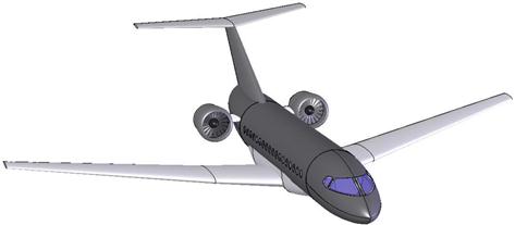
The cruciform tail configuration is often resorted to if it is desirable to feature aft podded engines. A wide range of aircraft use this tail arrangement, ranging from bombers such as the B-1B Lancer, the twin turboprop passenger transport aircraft Handley Page HP-137 Jetstream, or the now obsolete Sud-Est Caravelle, a classic early commercial jet transport aircraft. The Dassault Falcon family of business jets also features this tail configuration. NACA research on cruciform tails can be found in NACA reports TN-2175 [8] and RM-L54I089, among others. An example of a cruciform tail is shown in Figure 11-28.

The cruciform tail is a practical solution for an aft podded engine configuration and one that will result in lower structural loads than the T-tail (see later). It is also practical for freight aircraft designed to allow the empennage to be swung open for loading and unloading through the rear fuselage (as is the T-tail). Depending on the position of the break in the fuselage, a conventional HT might hit the wings when swung open and limit the allowable swing angle. Of course, there are conventional tail airplanes such as the four-engine Canadair CL-44 that show this is not necessary as it depends on the location of the opening and length of the fuselage. For such a configuration, the HT sits above the exhaust from the jet engines, as shown in Figure 11-29. The lower part of VT is exposed to “clean” airflow at high, post-stall AOA, improving spin recoverability. The position of the HT creates limited endplate effectiveness.
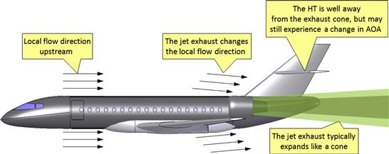
FIGURE 11-29 The cruciform tail configuration brings the HT out of the jet exhaust, although it may still be affected by a change in AOA on the tail with thrust setting.
Among drawbacks are higher torsional loads than for the baseline configuration (the conventional), which results in a heavier structure (albeit lighter than T-tail). Also, the VT must feature structural reinforcement to allow the HT to be mounted to it. As a consequence, this configuration will be heavier than the baseline tail, assuming identical size and shape of the tail surfaces. Another drawback of this configuration is that the upper part of the rudder is not fully exposed to “clean” airflow during spin recovery. Additionally, the configuration requires a sectored elevator (i.e. a sector of the root of the elevator is removed) to allow the rudder to deflect freely, or the rudder must be split in the area of the HT for the same reason. This requires additional manufacturing steps that could increase the cost of production of the rudder (or elevator). Furthermore, the configuration has higher interference drag.
11.3.3 T-tail
T-tails have been common on aircraft since the mid-1960s, when they appeared for the first time on a commercial passenger transport aircraft – the Boeing B-727. The concept was tested by NACA as early as 1954 [9,10], but has since been studied by NASA and other scientists in multiple publications. The configuration is considered by many to be stylish, a feature of great importance to the marketability of aircraft. Besides commercial transports, T-tails are very common on business jets, where they are more common than the conventional tail. Business jets ranging from the early Gates Learjet 25 through to the Gulfstream G650 feature the configuration. In the GA industry several aircraft feature the configuration. The best-known among smaller such aircraft are the twin-seat, single-engine trainers Piper PA-38 Tomahawk and Beech Model 77 Skipper. T-tails can also be found on larger twin-engine turboprops, such as the Beech 1900. Additionally, T-tails can be found on a range of sailplanes. An example of a T-tail is shown in Figure 11-30.
Among the advantages is that the tail leaves the rudder un-blanketed at post-stall AOA, giving the rudder a greater spin recovery potential (see Figure 11-31). The reader must be mindful of the shortcomings of the figure, which is a simple representation of an otherwise highly complex flow phenomenon. The flow field near the tail is dependent on the actual AOA and geometric features such as separation of wing and HT and shape of the fuselage. Figure 11-31 shows the aircraft at an AOA beyond deep-stall, discussed below. Additionally, as stated earlier, spin and spin recovery are complicated and an un-blanketed rudder is only part of what makes an airplane recoverable. Another advantage of the T-tail configuration is that it lends itself perfectly to aft podded engines, as are so common among business jets. If the VT is swept aft, which is also the norm for high-speed aircraft, an additional tail arm can be gained by placing the HT on top of the VT. As a consequence the tail can be slightly smaller than the baseline tail. Additionally, the endplate effect the HT gives to the VT can be utilized to reduce the size of the vertical tail, which allows for drag reduction (albeit modest). The high position of the HT effectively places it in a relatively undisturbed air, although this primarily holds true at low AOA. On sailplanes, where low drag is of utmost importance, placing the tail in undisturbed air is essential because this helps maintain NLF on their surfaces.
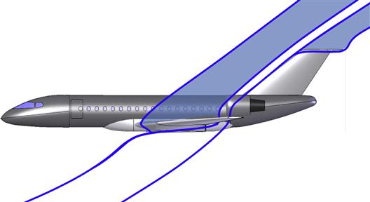
FIGURE 11-31 A schematic of a T-tail aircraft post-stall at a high AOA, showing the turbulent wake from the wing does not blanket the VT (see text for more details).
There are several disadvantages of this configuration. The high-mounted HT, coupled with the presence of the VT, can generate a substantial asymmetric lift in yaw. This results in high torsional loads that are reacted at the top of the fin and eventually by the fuselage. This torsion is compounded by the torsion from the VT that simultaneously results from the yaw, making the loads much higher. This impacts the structure of both the VT and the fuselage, causing an overall increase in its weight. The high mass of the HT mounted at the tip of the VT reduces the tail’s natural frequency of oscillation, effectively lowering its flutter speed. This may have to be remedied by additional structure to increase the tail’s stiffness, further increasing its weight. Maintenance is impacted as repair stations will have to accommodate technicians working on the tail high above the ground.
One of the configuration’s primary disadvantages is that the tail may end up inside the wing wake at stall or post-stall (see Figure 11-32). The figure shows how the HT may ultimately come to rest inside the highly separated wake from the wing. Therefore, the elevator authority is severely diminished and may even disappear. Note that the figure does not necessarily depict the only attitude possible – some aircraft have been reported descending mostly horizontal at a high AOA, others in a more nose-down attitude. This is a very serious condition that in the extreme case can render the aircraft incapable of dropping the nose and recovering from the stall. It is recognized as a “deep-stall” and has caused multiple development and operational vehicles to crash with fatal consequences. It is one of two important reasons why commercial transport aircraft with T-tails always feature “stick-shakers” or “stick-limiters” for the elevator control yoke in the cockpit. That way, the pilot cannot stall the airplane inadvertently.
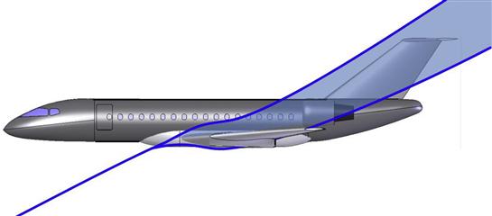
FIGURE 11-32 A T-tail aircraft at a high AOA, showing the HT inside the wing wake, causing the “deep stall” phenomenon.
To understand how the deep-stall phenomenon can affect an airplane with a T-tail, consider Figure 11-33, which shows a typical T-tail aircraft. Again, the three curves represent the Cm for the complete aircraft with different elevator deflections. The top curve represents Cm with the elevator deflected 20° TEU, the center curve depicts the elevator in a neutral position, and the bottom depicts the elevator deflected 15° TED. The three trim points in the pre-stall region are similar to those of Figure 23-19.
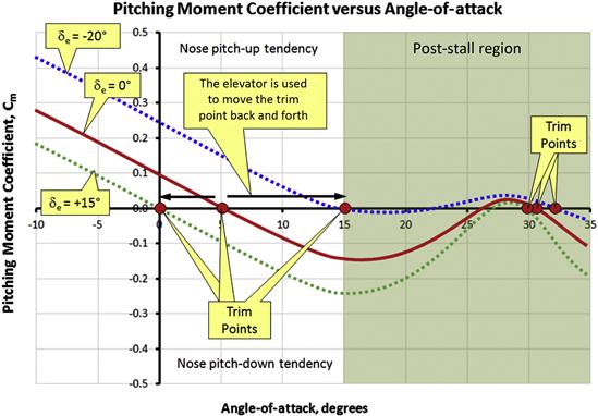
Now consider the right side of the graph of Figure 11-33, which is shaded and titled the “Post-stall Region.” The airplane being represented stalls around 15°. If it is driven to stall abruptly, this would be accompanied by angular momentum about the pitch axis, which might rotate it to an α greater than 15°. If the angular momentum is high enough, the pitch angle would be driven farther to the right to an even higher α, where some strange things begin to happen.
The first thing to happen is that the negative slope of the aircraft becomes positive (i.e. unstable). This positive slope would be realized as a tendency to increase the α further. This is caused as the HT enters the wing wake, which suppresses its effectiveness. Consequently, the natural instability of the fuselage (as it is a body of revolution) will destabilize the vehicle, causing the curves to approach the horizontal axis (around 16°–18°). Eventually, they intersect it and ascend into the positive part of the graph before descending back down as the tail moves out of the wake due to the excessively high AOA. This tendency is common among T-tail aircraft. The consequence of this behavior (which is caused by the tail entering the highly turbulent wing wake as shown in Figure 11-32) is that each curve now has a corresponding trim point around an AOA of 30°–32°. These points pretty much cover the entire travel of the elevator. The problem with this is that the reduction in elevator authority at those AOAs, which are noticeable by the closeness of the three curves, renders the aircraft practically uncontrollable in pitch. It won’t matter how much the pilot moves the yoke forward or back, the elevator deflection on its own cannot bring the airplane out of this equilibrium condition. Consequently, it will stay there at this high AOA, fully stalled and uncontrollable as it descends rapidly, eventually crashing. For some aircraft, applying full engine power might help nudge it out of this stable post-stall AOA, although aircraft with jet engines may experience a flame-out to further compound the situation. The prototype of a new design that features a T-tail should not be stalled in flight testing without a spin recovery chute, in case it is susceptible to this phenomenon.
The history of aviation is wrought with deep-stall accidents in T-tail aircraft. A Gloster Javelin was lost on June 11, 1953, due to this phenomenon [11], killing the pilot. On March 23, 1962, a Handley Page Victor crashed killing two of the crew of five and two people on the ground [12]. On October 22, 1963, a BAC 1-11 crashed on a test flight due to deep-stall killing all seven occupants [13]. Coincidentally, the very same day a Tupolev Tu-134 crashed due to the same cause [14]. On June 3, 1966, a Hawker Siddeley HS-121 Trident crashed on a test flight, killing the crew of four [15]. These are but a few of a long list of such accidents in which a T-tail was the contributing factor.
11.3.4 V-tail or Butterfly Tail
Research on V-tail configurations dates back to 1931 with the publication of an anonymous paper that discussed the so-called Rudlicki V-tail.1 The configuration combined the three surfaces of the conventional tail into two surfaces that form a distinct V (see Figure 11-34). This way the functionality of a typical single rudder surface and two elevator surfaces is combined in two surfaces that are called ruddervators. The ruddervators are deflected in a manner that effectively recreates the functionality of the rudder and elevator (see Figure 11-35).
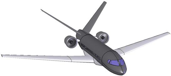
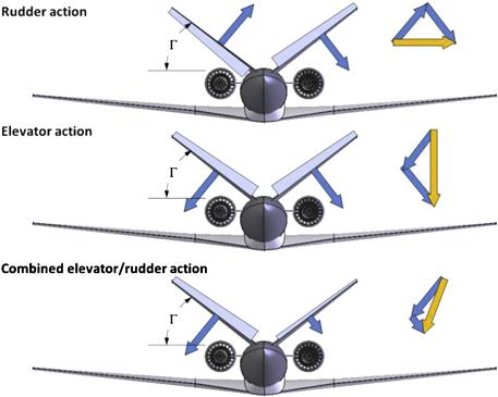
FIGURE 11-35 How ruddervators are used to generate the primary functionality of the conventional rudder, elevator, and combined action.
V-tails can be found on a wide range of aircraft, ranging from sailplanes, to propeller and jet aircraft. Some of these are shown in Table 11-3. Among sailplanes is the Glasflügel H-101 Salto aerobatic sailplane. The best-known GA aircraft featuring a V-tail is the four-seat, single-engine Beech Model 35 Bonanza, which was first introduced in 1947. Two brand-new aircraft designs appeared in 2007, the Cirrus SF50 Vision and the Eclipse-jet, both being single-piloted personal jets, which feature a single Williams FJ33 turbofan mounted in a pod on top of the fuselage. The Northrop Grumman RQ-4 Global Hawk is a well-known unmanned aerial vehicle (UAV) that features V-tails. Additionally, the Fouga CM-170 Magister, a twin-engine, two-seat military trainer, introduced in 1948, features a V-tail.
TABLE 11-3
Selected Aircraft Featuring V-tails
| Aircraft type | Comment |
| Beechcraft V35 Bonanza | Single-engine, four-seat GA aircraft. Produced in large numbers. |
| Fouga CM-170 Magister | Twin-engine, twin-seat military trainer (195X). Produced in large numbers. |
| Potez-Heinkel C.M. 191 | Based on the Fouga Magister. Prototypes only. |
| The Zipper | Ill-fated aircraft. |
| F-117 Nighthawk | Military fighter, stealth configuration, fly-by-wire. |
| Global Hawk | UAV. |
| Microjet | Twin-engine, twin-seat jet trainer candidate. Only prototypes built. |
| Dale AE Weejet 800 | Prototype only. |
| P-63 Kingcobra | A Kingcobra fitted with a V-tail for testing purposes. Prototype only. |
| Eclipse V-jet | Prototype GA personal jet. Single-engine jet. Prototype only. |
| V-jet | Developed in participation with Williams International. Prototype only. |
| Cirrus SF50 Vision | Prototype GA personal jet. Single-engine Williams FJ33 jet. |
| Hütter 30 GFK | Sailplane. |
| Musters HKS 1 | Sailplane. |
| Schleicher Ka 3 | Sailplane. |
| Greif 1a (FK 1) | Sailplane. |
| Greif 2a (FK 2) | Sailplane. |
| Schreder HP-12 | Sailplane. |
| Schreder HP-18 | Sailplane. |
| Start & Flug H101 Salto | Sailplane, aerobatic. |
Considerable research was done on such tails by NACA in the 1940s and multiple reports are available from the online NASA Technical Report Server [16]. For instance, the NACA reports TN-1369 [17], TN-1478 [18] and R-823 [19] should be very helpful to the designers of V-tail aircraft. The last one (R-823) was particularly helpful to the author of this book during such a development program.
Let’s consider the advantages of V-tails as stated by NACA R-823, where comparison is made to the conventional tail. First, there is less interference drag because the V-tail has fewer fuselage-tail junctures. Second, there is less tendency for “rudder locking,” a phenomenon discussed in Section 11.2.11, The dorsal fin. Third, the higher location of the tail surfaces reduces required elevator deflection as the center of pressure is above the fuselage and therefore the drag component of the deflected ailerons will increase the nose pitch-up moment. This is depicted in Figure 11-36.

The pitch-up moment M can be written as: M = FV· a + FH·b, where FV is vertical component of the resultant force acting on the V-tail, FH is horizontal component, and a and b are the arms shown in the figure. The corresponding moment for a conventional tail would be closer to FV·a. Additionally; the surfaces extend farther out of ground effect than the conventional tail, making the tail more effective during T-O and landing. Fourth, for amphibious aircraft the tail will most likely be out of the spray during the T-O, making it more effective. Fifth, the tail is out of the wake of the wing and canopy in high-speed flight and therefore there is less chance of tail buffeting. Sixth, there are fewer tail surfaces to manufacture.
A V-tail is a great configuration for aircraft equipped with single jet engines and allows them to be mounted in a pod on top of the fuselage, on the aircraft’s centerline. Two recent examples of such a design solution are the Cirrus SF50 Vision and the Eclipse-jet.
The following disadvantages are cited in NACA R-823 [19]. First, there is a possible interaction of elevator and rudder control forces. For instance, during a cross-wind landing the pilot might use the rudder pedals to side-slip the airplane on final approach. Since this would cause a TEU deflection in one of the ruddervators and a TED in the other one, the elevator stick-forces would be affected when compared to those with the rudder neutral. Second, there is a possible interaction of elevator and rudder trimming, when trim tabs are deflected to large angles. Third, the control system requires a special treatment of the control inputs. This is done using a device called a control system mixer (see Figure 11-37). Fourth, it results in greater loads on the tail and fuselage, which tends to increase structural weight. This is caused by the fact that the V-tail must serve as the HT and the VT. This requires its size to be larger than if it only served one purpose. Consequently, during maneuvers, such as yawing, a larger force will be generated, which of course requires stouter and, thus, heavier structure.
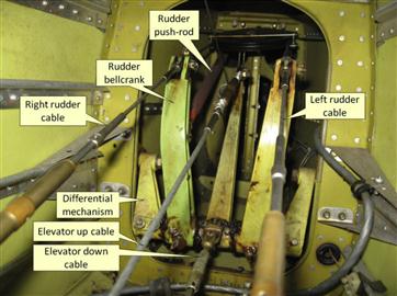
But there are other shortcomings not mentioned by R-823 [19]. First is that the application of rudder will cause the airplane to roll in a direction opposite to the intended bank. To understand what this means, consider a pilot wanting to execute a turn to the left. To accomplish this, the pilot will roll the left wing down. This causes the right wing to be raised and, consequently, it will move through an arc with a greater radius than the left wing. This makes it move faster through air than the left wing. It follows it generates higher drag than the left wing, and this causes a tendency for the nose to point to the right, even though the heading is changing to the left. This phenomenon is known as an adverse yaw and the pilot simply cancels it by stepping on the left rudder pedal. If we observe the aircraft from behind as this happens, we would see the pilot action forcing the tail to the right, in the process moving the nose to the left (the intended direction). For some aircraft the pilot actively corrects the turn in this fashion, while for others there is less need to. The preceding description is not a consequence of a V-tail, per se, but needs to be kept in mind when considering the following effects.
Now consider Figure 11-38, which compares a rudder input for a V-tail and an inverted V-tail. The upper image shows the ruddervators of a V-tail deflected to produce a nose-left yaw (move the tail to the right). The left ruddervator is deflected TED and the right one is deflected TEU. The resulting force vectors on the tail surfaces give rise to a tendency for the aircraft to roll to the right, which is the opposite of the intended turn. Such tendency is called an adverse roll.

FIGURE 11-38 The difference in yaw response of a V-tail and an inverted V-tail. The intent of the pilot is to bank to the left and coordinate the turn with the rudder. If high rudder deflection is required, a conventional V-tail will tend to rotate the plane out of the turn, whereas an inverted V-tail will rotate it into the turn.
Then, review the lower image in Figure 11-38. It shows how the ruddervators on an inverted V-tail would have to deflect in order to move the tail to the right. The left ruddervator is deflected TEU and the right one TED. The resulting force vectors on the tail cause a tendency that would roll the aircraft to the left – in the intended direction. In short, the inverted V-tail helps the pilot execute the turn. The short version of the above is: a V-tail rolls the airplane out of a turn. An inverted V-tail rolls the airplane into the turn. The latter is more desirable. Such tendency is called a proverse roll.
It is an additional drawback that the airplane’s rotation about the pitch axis is due to the vertical component of the lift acting on the V-tail. For this reason, a larger tail is needed. There is a control system interaction, such that stepping on the rudder pedals may cause a nose pitch-up or -down moment, depending on the geometry of the tail and the airfoil. This may call for ruddervator deflection differentials to be built into the control system. For example, such a differential control may result in deflections in which TED ruddervator deflects −6° while the TEU ruddervator deflects +10°. And finally, an important attribute of a V-tail is that it increases the dihedral effect of the aircraft. Consequently, a reduced Dutch roll damping should be expected as well as more of a “rolling” type of Dutch roll. Such aircraft, in particular high-flying jets, may have to feature a yaw damper (which of course all high-flying jets feature anyway).
Simplified Theory of V-tails
Reference 19 lists a number of expressions that are handy in the design of V-tails. The reference presents the following set of experimentally verified formulations to help with the design of the configuration (derivation is provided in the reference document):
Lift curve slope of the V-tail:
![]() (11-29)
(11-29)
Elevator authority of the V-tail:
![]() (11-30)
(11-30)
Side force slope of the V-tail:
![]() (11-31)
(11-31)
Rudder authority of the V-tail:
![]() (11-32)
(11-32)
where
![]() lift curve slope of the planform at a zero dihedral
lift curve slope of the planform at a zero dihedral
τ = control effectiveness parameter
K = the ratio of sum of lifts obtained by equal and opposite changes in angle-of-attack of two semi-spans of tail to lift obtained by an equal change in angle-of-attack for complete tail
Formulas for the control effectiveness parameter, τ, are given in the reference document, but it is a function of the tail and wing geometry, the V-tail dihedral, and elevator authority, to name a few.
11.3.5 Inverted V-tail
The inverted V-tail (Figure 11-39) shares many of the pros and cons of the V-tail, but has seen far less use in the industry. The best-known example of its use is the homebuilt single-seat monoplane Aerocar Mini IMP, although some versions featured a vertical tail addition resulting in an inverted Y-tail (see later). The General Atomics Predator, an unmanned military aircraft, also has an inverted V-tail, although some would object to that definition as it also has a vertical fin between the two outboard tails – sort of like a “collapsed” inverted Y-tail. Additionally, the Elbit Hermes 90 unmanned aerial vehicle (UAV) features an interesting inverted V-tail on an elevated tailboom.
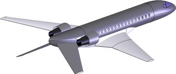
A great advantage of the inverted V-tail configuration is the proverse roll tendency discussed in the previous section. Its greatest drawback is that its tips reduce the T-O rotation and flare potential of the aircraft. For this reason, the tail must be mounted high on the fuselage and long main landing gear legs are likely to be required to improve the rotation capability of the airplane.
11.3.6 Y-tail
From a certain point of view, the Y-tail (Figure 11-40) is a variation of the V-tail. One might say it is a V-tail with an additional vertical surface. Like the V-tail it requires a ruddervator control mixer (otherwise it is just an inverted conventional tail with the horizontal featuring a very high dihedral). However, sometimes a rudder is also mounted on the vertical ventral fin on the bottom, giving the aircraft increased rudder authority. The most notable aircraft that feature this tail are the General Atomics Predator B and the cancelled LearAvia Lear Fan 2100 aircraft.
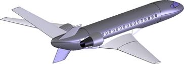
Among the tail’s advantages is an improvement to the directional stability and Dutch roll damping provided by the vertical element of the tail and this presents an improvement over the conventional V-tail configuration. This allows for a shorter-span V-tail. Even a relatively short-span vertical element can provide substantial improvement in the Dutch roll damping. A major drawback with the configuration is that it presents a serious challenge to rotation during T-O and flare during landing. This can put a significant limit on the permissible span of the vertical surface, reducing its ability to improve directional stability and Dutch roll damping. However, as usual, the practicality of a particular tail configuration ultimately depends on the general geometry and, as the aforementioned aircraft indicate, a Y-tail can be successfully featured.
11.3.7 Inverted Y-tail
Many of the pros and cons of the Y-tail also apply to the inverted Y-tail. However, the tail would bring about great improvements in stall recovery as the down-pointing tail feathers will pitch into unseparated flow, which contrasts the Y-tail’s tendency to rotate into the wing wake. By far the best-known aircraft that features an inverted Y-tail is the cold-era fighter McDonnell Douglas F-4 Phantom, although some would argue it is a conventional tail configuration whose HT has a large anhedral. The greatest detriment for the configuration is shown in Figure 11-41, in the case of a conventional jetliner in which it would severely limit the ability of the aircraft to rotate for T-O or landing.

11.3.8 H-tail
The H-tail (Figure 11-42) is a good solution when the overall height of an airplane is an issue and a single VT is simply too tall. It is a good configuration for twin-engine propeller aircraft as well, providing a means to supplement the restoring yawing moment required to balance the asymmetric moment caused in a one engine inoperative (OEI) situation. By placing the two VT surfaces inside the propwash of each engine, should one engine be lost only one of the two surfaces experiences a reduction in dynamic pressure. Sometimes, the VT is installed with a slight incidence to further supplement the restoring yawing moment (e.g. Breguet Br-695), but this may not be required, as the propwash tends to follow the shape of the fuselage and be bent, placing the VT at an AOA that promotes the generation of this restoring yawing moment.

Military aircraft of the past often featured an H-tail, where the vertical surfaces were of a very small AR, frequently in the 1.0 range. The benefit of this is a VT surface that stalls at a very high AOY, which helps preventing the airplane from experiencing rudder lock (see Section 11.2.11, The dorsal fin). For this configuration a dorsal fin is not necessary. The configuration also increases the efficiency of the horizontal tail through endplate effects. This effect promotes a uniform lift distribution by eliminating lift drop-off at the tip and allows the size (and thus weight and drag) of the HT to be somewhat reduced (see Section 10.5.8, Endplate wingtip).
An important detriment of the configuration is reduced flutter speed. This is caused by the reduction in the natural frequency of the HT because of the mass of the VT being placed at its tip. This reduction in flutter speed must be improved by stiffening the HT, which will increase the overall weight of the configuration. The Lockheed Model 14 Electra, a twin-engine, 10-passenger, transport aircraft developed in the 1930s, is a classic example of an aircraft featuring an H-tail that suffered fatal accidents due to tail flutter.2 It is not clear whether this was due to the rudder fluttering (which can happen on all aircraft) or the HT/VT combination itself, although this does not change the above statement. An additional flaw is that the tail experiences peculiar air loading scenarios at high AOY that may also call for an increase in structural weight. The configuration will also require the rudder control system to feature a split so both rudders can move in harmony, which increases control system complexity. And finally, there is higher interference drag and the lift curve slope of the tail is small due to the small AR.
11.3.9 Three-surface Configuration
A three-surface configuration consists of a main wing with a foreplane and a horizontal tail. The foreplane is so called as it is positioned ahead of the wing. The horizontal tail is positioned aft of the main wing identical to that of the conventional configuration. The idea with the configuration is to place the CG such that all lifting surfaces can contribute to lift, making the configuration more efficient through a reduction in lift-induced drag. Of course, this is offset by an increase in interference drag.
The main lifting surface can consist of one or more separate wings. In this context, a biplane with two stabilizing surfaces (effectively a four-surface aircraft) should be considered a three-surface aircraft, because the intent of the two main wings is to generate lift and not stabilizing moments. Modern times have only seen a few examples of such aircraft making it to the production stage. However, a number of three-surface biplane configurations were developed in the early part of the twentieth century. Among the first was the Voisin 1907 biplane, also called the Voisin-Farman No. 1 after the French aviator and aircraft designer Henri Farman (1874–1958). Farman designed and built the Henri Farman biplane, which first flew in 1909. It is also known as the Farman III. Other airplanes include the Bristol Boxkite, which first flew in 1910, and the Cody Biplane No. 3, which first flew in 1911. At least three aircraft designed by Joseph Albessard featured monoplanes. These were the Albessard 1911, Albessard 1912, and the Albessard Triavion [20], which flew for the first time in 1926. All are peculiar aircraft with the main wing in front, a smaller wing in the middle of the fuselage, and a smaller yet horizontal tail located aft.
The best-known modern three-surface aircraft is the Piaggio P180 Avanti, an Italian twin-turboprop business-class transport aircraft that carries up to 10 occupants. The airplane is a truly unique design intended to compete with business jet aircraft and is touted as the fastest twin-turboprop ever built, capable of 402 KTAS at 38,000 ft (M ≈ 0.70).3 That aside, the manufacturer claims the three-surface configuration results in 34% less drag than comparable turbofan aircraft and offers 40% improvement in fuel consumption. The aircraft has a flap on the forewing that deflects trailing edge down (TED) when the flaps are deployed to counter the resulting pitch-down moment. The elevator is located on the aft surface. This arrangement helps keep control system complexity manageable.
The configuration calls for more localized structural reinforcements and more interference drag, offsetting the reduction in lift-induced drag somewhat. The foreplane also places the inboard wing in downwash on, reducing the effectiveness of the wing further. Furthermore, considering the aircraft in Figure 11-43, the foreplane tip vortices might cause a distortion in flow into engine and cause detrimental asymmetry in the compressor loading.
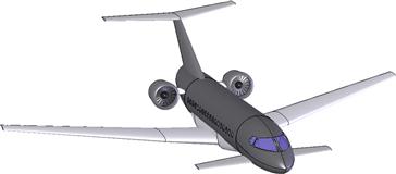
11.3.10 A-tail
The A-tail (Figure 11-44) is a variant of the inverted V-tail, so the reader is referred to Section 11.3.5, Inverted V-tail, for further discussion of pros and cons. The configuration is already used in UAVs such as the AAI RQ-7 Shadow and UAV Factory Penguin B UAV, although it has seen very limited use in aircraft that carry people. The Vogt LO-120 ultralight is an example of a small experimental aircraft, as is the Advanced Aero LLC’s Inverted V-tail Technology Demonstrator. The former is exceedingly rare and the latter has not flown yet, although the configuration experienced limited flight testing on a heavily modified Sadler Vampire experimental light plane in 2010.

11.3.11 Twin Tail-boom or U-tail Configuration
The twin tail-boom configuration has seen extensive use in the history of aviation, where it has been used for both large and small aircraft. Examples of GA aircraft include the Cessna 337, of which some 3000 aircraft were built; Adam A500 and A700, and others. Among famous military aircraft are the Northrop P-61 Black Widow, Lockheed P-38 Lightning, and the North American Rockwell OV-10 Bronco. The latest entry of such a configuration is the South African AHRLAC twin-seat reconnaissance aircraft. A typical GA implementation of this configuration is shown in Figure 11-45. Although the version shows extension on the lower VT, the tail effectively forms an arrangement that can be described with the letter U (hence the U-tail name).
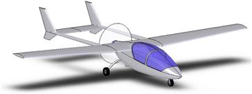
For propeller configurations, the HT is often placed in the propwash, giving it boost for soft-field T-O maneuver and good responsiveness. However, this is not always the case. A great advantage of the configuration for smaller aircraft is that the tail-booms form an obstruction making it hard for people to accidentally walk into the prop. Pros and cons of the configuration are detailed in Section 11.3.8, H-tail.
Inverted U-tail
An inverted U-tail refers to a configuration in which the HT is placed on the top of the VT (see Figure 11-46). This configuration is used on the North American OV-10, Adam A500, and Adam A700. On propeller aircraft, it places the HT outside the propwash, reducing its drag, but also eliminating a propwash boost over it.

11.3.12 Canard Configuration
A canard configuration is one in which the horizontal stabilizing surface is placed in front of the main wing (see Figure 11-47). This placement generates a destabilizing pitching moment, which contrasts the stabilizing moment generated by tail-aft configurations. The configuration actually dates back to the early days of aviation. As an example, the Wright Flyer, the first heavier-than-air airplane, was a canard. The configuration sporadically appeared in various experimental designs throughout history and got its greatest boost in the early 1970s with advent of the Rutan VariEze and LongEze homebuilt aircraft. Canard aircraft are discussed in more detail in Appendix C2: Design of canard aircraft, so the discussion will be limited here.
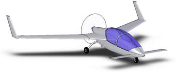
One of the most touted advantages of the canard configuration is stall-proofing which refers to a characteristic in which the canard stalls before the main wing. This lowers the nose and prevents the main wing from stalling. This is often presented as an inability of the airplane to stall. In fact this is an inaccurate description; it is indeed possible to stall the main wing. For instance, by an abused stall entry. For instance, it is possible to drive the airplane to a high enough AOA to stall the main wing using high rotational momentum. However, the term stall-proofing is generally taken to mean a normal 1 knot/sec deceleration approach to stall. If this deceleration is maintained, such airplanes are indeed designed to gently drop the nose before the main wing stalls. Under those circumstances, the canard can be considered stall-proof.
Another advantage of the configuration is that in stable level flight the lift of the canard points upward, in contrast to a downward force generated by the conventional tail-aft configuration. This means the canard contributes to the total lift of the aircraft, rather than the weight (i.e. the downward-acting force). Consequently, it is commonly maintained the vehicle can be flown at a lower AOA in cruise, which means less lift-induced drag, making the concept more efficient than conventional aircraft.
One of the drawbacks of the configuration is that it requires higher T-O airspeed than a tail-aft configuration and, thus, has longer runway requirements. This is a direct consequence of the stall-proofing. It leads to a configuration whose minimum speed is higher than if the main wing were indeed allowed to stall. In simple terms this means the airplane must accelerate to a higher rotation speed during which it covers greater distance. Its landing distance is longer for the same reason.
Another drawback is that the generally compact size of canards results in a tail arm that tends to be smaller than similarly sized conventional aircraft. This must be made up for by a larger stabilizing surface or, more commonly, by sweeping the main wing aft to move the MGC farther away from the canard – thus increasing the arm. Generally, while the popular canard configurations (LongEze, Cozy, and others) display good flight characteristics, their directional stability is often weak (for instance see Ref. [21]). This is due to the short tail arm of the winglets at the tip of the wing. Here, the aft-swept wing is one way to improve this.
While stall-proofing has come to mean an automatic stall recovery, the stall may result in a large nose-drop, depending on how aggressively it is performed. This is due to the fact, and as is pointed out by Larrabee and Abzug [7], that the angular pitch rotation following the stall increases the AOA on the canard and can delay stall recovery until a steep nose pitch-down attitude is achieved. They point out that an argument can be made that conventional tail-aft aircraft can also recover automatically with the appearance of sudden upwash on the HT as the wings’ downwash disappears at stall.
Other drawbacks of the configuration are a reduction in forward and downward visibility caused by the canard which also reduces the effectiveness of the main wing. This must be made up by flying the vehicle at a higher AOA and, thus, a greater lift-induced drag than if the downwash were not present. This cuts into any advantage offered by the positive lift of the canard. Additionally, the reduction in the section lift coefficients of the main wing (that result from the downwash) increases the margin between the canard stall and the subsequent wing stall – something that may further increase the minimum speed of the vehicle. The downwash also means the outboard wing generates higher lift than it would in its absence – so the wing bending moments are increased.
11.3.13 Design Guidelines when Positioning the HT for an Aft Tail Configuration
It has been known for a long time that the location of the horizontal tail with respect to the wing of conventional aircraft configuration plays an essential role in the handling characteristics near or at stall. Such characteristics are only problematic if the airplane inherits a tendency to pitch-up uncontrollably near stall. Such problems can be caused by the distortion of the flow field because of the highly separated flow emanating from the wing and fuselage at high AOAs. The separated flow field reduces the tail effectiveness, in the worst-case scenario, enough to make recovery impossible. This has already been discussed in terms of T-tails (see Section 11.3.3, T-tail). It has also been discussed that T-tails are considered by many to offer an appealing appearance, making them an attractive option to the aircraft designer. However, it is imperative that the designer is aware of both this short-coming and its possible solution, for instance the ventral fin (see Section 11.2.12, The ventral fin).
The pitch-up problem was studied in NACA R-1339 [22] and showed that the wing sweep can have a large impact on the nonlinearity in the pitching moment curve near stall. However, this may be complicated by the presence and location of the HT (see Figure 11-48). In the absence of the tail the figure shows the swept wing on its own becomes unstable. However, with a T-tail, the same wing will become stable, only after crossing the horizontal axis. This, in turn, creates another trim point (here at approximately AOA = 29°), from which the configuration may not recover (deep-stall).
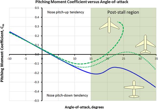
FIGURE 11-48 Pitching moment curves, for example swept-back and straight wing configurations. The curve for the swept-back wing is seen to wander into the upper part of the graph at higher AOAs. This is indicative of a nose pitch-up tendency characteristic of swept-back wings.
Straight wings with T-tails, on the other hand, may cause nonlinearities that are restricted to a small range of AOAs near stall. For this reason, such aircraft with the horizontal tails mounted high above the main wing may experience reduced stability but not detrimental instability. And they are less likely to have a trim point in the post-stall region. Therefore, the horizontal tail of such aircraft can be sized with trim capability throughout its operational range. In spite of this, this author recommends the designer considers the possibility of deep-stall tendency, either by wind tunnel testing or by a stall evaluation of a radio-controlled model. The former should be required for all aircraft intended to carry people for commercial purposes, the latter can be considered an option for smaller manufacturers or homebuilders. As stated in Ref. 23, the effect of the fuselage may be hard to predict otherwise and can easily devolve into a major design problem, in particular for low-AR wings with thin airfoils.
Swept-back wings suffer flow separation at lift coefficients well below that CLmax and are either unstable or marginally stable through stall. Therefore, configurations with swept-back wings must be treated in a much different and more stringent way than the straight wing and should be wind tunnel tested at all cost. Reference 23 is a compilation of many sources and provides the high-AOA properties of a large array of configurations, with straight and swept wings, with and without fuselages and various high-lift devices.
The pitch-up problem was also studied in NACA TN-1093 [23]. While focusing on the wing planform, the investigation, like that of Ref. [23], reaffirms that while the wing sweep can have a large impact on the nonlinearity in the pitching moment curve near stall, the impact of taper ratio and aspect ratio are imperative. In order to prevent instability a large AR should have reduced leading edge sweep. A low taper ratio aggravates tip stall and is thus detrimental to the stability. All of this impacts the selection of the HT location because it must remedy the instability issues. The combined effect of AR and leading edge sweep from Refs 23 and 24 are depicted in Figure 11-49.
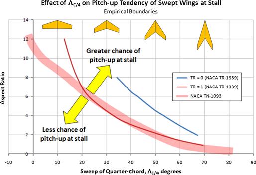
FIGURE 11-49 Empirical pitch-up boundary for a swept-back wing. Reproduction based on Refs [22] and [23].
The pitch-up problem was studied in NASA TM-X-26 [24] using low-aspect-ratio wings (AR ranged from 1.55 to 3.0) with substantial leading edge sweep, such as those more commonly associated with fighter aircraft. While the results, in general, apply only to aircraft with AR ranging from 2 to 5, they give important clues to the trends when comes to the positioning of the HT behind the wing. This is shown in Figure 11-50, which is a reproduction of Figure 3(b) in the reference document. The designer of tail-aft aircraft should compare the intended location of the tail in order to evaluate the probability of an uncontrollable pitch-up at stall. A horizontal tail positioned in Region A or B will likely call for aerodynamic fixes in the form of ventral fins.

FIGURE 11-50 Recommended placement of the HT behind the wing. Reproduction based on Ref. [24].
11.4 The Geometry of the Tail
In short, the purpose of the tail is to supply the vehicle with adequate pitch and yaw stability, which, of course, begs the question: how big should the tail surfaces be and where should they be located in order to provide “adequate” stability? In this section we will begin to answer the question by establishing means to evaluate tail geometry and then present some historical reference values of selected aircraft. In the next section we will close the loop by presenting methods that allow the size and location of the tail to be estimated.
Consider the simplified airplane shown in Figure 11-51. The fuselage extending from the wings’ quarter-chord plane to the quarter chord of the horizontal or vertical tail (denoted by the dashed lines) has been approximated by a frustum. The stabilizing surfaces have been approximated by flat plates. We will now use the abbreviations HT and VT for the horizontal and vertical tails, respectively. The area of the HT, SHT, is defined as the product of its average chord, CHT, and span, bHT. Similarly, the area of the VT, SVT, is defined as the product of its average chord, CVT, and span, bVT. Then we define the horizontal tail arm, lHT, as the distance from the quarter chord of the wings’ MGC to the quarter chord of the MGC of the HT. The vertical tail arm, lVT, is defined in a similar manner.
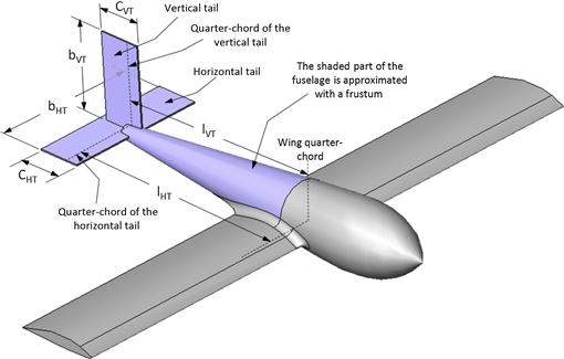
Note that the combination of the horizontal and vertical tail with its supporting structure is commonly referred to as the “empennage.”
11.4.1 Definition of Reference Geometry
Just like for the wing reference area, the reference area for both the horizontal and vertical lifting surfaces must be defined. Figures 11-52 to 11-55 show how aircraft designers typically define the reference area; however, and this needs to be emphasized: the shaded regions may not be what the actual manufacturers did for these particular aircraft, just what would be a likely approach.

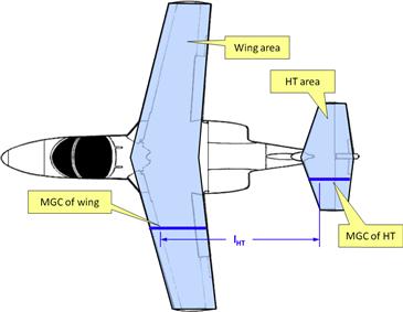
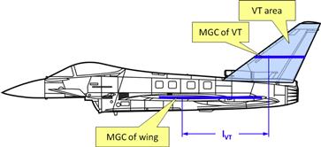
FIGURE 11-54 Definition of VT area and tail arm for the Eurofighter EF-2000 Typhoon. (Source: www.wikipedia.org)
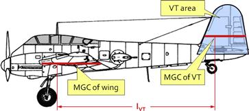
FIGURE 11-55 Definition of VT area and tail arm for the Messerschmitt Me-210 Hornisse. (Source: www.wikipedia.org)
The distances lHT and lVT are defined to extend from the quarter chord of the MGC of the wing to the quarter chord of the MGC of the horizontal or vertical tails, respectively.
The aspect ratio of the HT is determined precisely like that of the wing; however, determining the AR of the VT is often confusing because the surface is in many ways a half a wing. This is not a problem though. The definition of the AR for the VT is straight forward as shown in Section 11.4.2, below.
11.4.2 Horizontal and Vertical Tail Volumes
The formulation of the static pitch and directional stability, using stability and control theory, leads to the occurrence of terms that have come to be called horizontal and vertical tail volumes. These non-dimensional ratios compare the product of the stabilizing planform area and its distance from the wing to the basic wing geometry, which is the product of either the reference wing chord and wing area or the reference wing span and wing area. It turns out that the value of this ratio can be correlated between classes of aircraft (see Section 11.4.4, Recommended initial values for VHT and VVT). We define the horizontal and vertical tail volumes as follows:
![]() (11-33)
(11-33)
![]() (11-34)
(11-34)
where
cREF = mean geometric chord, ft or m
bREF = reference span (e.g. wingspan)
If a desired value for the horizontal or vertical tail volume is known, Equations (11-33) and (11-34) can be used to extract a number of information, as will be shown in Section 11.5.
11.4.3 Design Guidelines for HT Sizing for Stick-fixed Neutral Point
It is the purpose of stability and control theory to determine the location of the stick-fixed neutral point and other stability-related limitations. Here, however, it is prudent to give some design guidelines, albeit only for the stick-fixed neutral point. The stick-free neutral point depends on the hinge moments of the elevator and, therefore, is a design concern later in the preliminary design.
It can be shown that the stick-fixed neutral point for aspect ratios in excess of 4 is mostly independent of its magnitude, but instead is mostly a function of the horizontal tail volume, VHT, defined by Equation (11-33). This is shown in Figure 11-56, which depicts how the VHT affects the location of the neutral point. The graph assumes the wing and HT only and symmetric airfoils for both.

FIGURE 11-56 Impact of horizontal tail volume on the location of the stick-fixed neutral point. It can be seen that above an AR = 4, the AR has minimal influence on the location of the neutral point.
As an example of how the graph in Figure 11-56 is read, assume an airplane whose VHT = 1.0. The airplane should be expected to have a stick-fixed neutral point of approximately 0.68. This may drop to 0.45 or so once the fuselage is added. In fact, the graph allows the VHT for a desired stick-fixed neutral point to be estimated. This is done using the following expression based on the curve fit in Figure 11-56:
![]() (11-35)
(11-35)
This expression can be used as a “first stab” estimation of the necessary VHT assuming no fuselage. The presence of a fuselage might move the hn some 0.1–0.15 forward, assuming the target VHT ranges from 0.4 to 1.0. The reader must be mindful that this estimation says nothing about handling – some aircraft may need smaller or greater VHT depending on other operational requirements.
EXAMPLE 11-4
Estimate a plausible VHT required for an airplane whose hn is expected to be close to 0.4 CREF including the fuselage.
Solution
Using Equation (11-35) and assuming that the stick-fixed neutral point, hn, of the wing-HT system will be close to 0.4 + 0.1∼0.5; therefore, the designer should initially shoot for a VHT close to:
![]()
11.4.4 Recommended Initial Values for VHT and VVT
One of the first tasks in the initial sizing of the aircraft is to determine candidate dimensions for the HT and VT. This can be easily accomplished by investigating the horizontal and vertical tail volumes of existing classes of aircraft. Raymer [1] presents the VHT and VVT for different classes of aircraft shown in Table 11-4.
TABLE 11-4
Candidate Horizontal and Vertical Tail Volumes per Class of Aircraft
| VHT | VVT | |
| Sailplanes | 0.50 | 0.02 |
| Homebuilt | 0.50 | 0.04 |
| GA – single-engine | 0.70 | 0.04 |
| GA – twin-engine | 0.80 | 0.07 |
| Agricultural aircraft | 0.50 | 0.04 |
| Twin turboprop | 0.90 | 0.08 |
| Flying boat | 0.70 | 0.06 |
| Jet trainer | 0.70 | 0.06 |
| Jet fighter | 0.40 | 0.07 |
| Military cargo/bomber | 1.00 | 0.08 |
| Jet transport | 1.00 | 0.09 |
(Based on Ref. [1])
Table 11-5 presents helpful reference data for the taper ratio and volumes of the horizontal and vertical tail for a number of classes of aircraft. These are based on measurements of three-views. The designer is strongly urged to compare the tail volume of own design to historical data of the kind presented below.

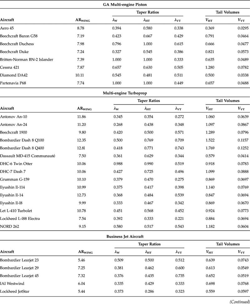
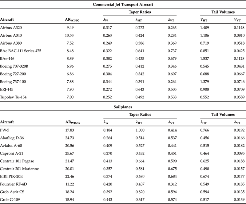
11.5 Initial Tail Sizing Methods
Unless other factors are considered of greater importance, the designer should always try to minimize drag. Since the bulk of the airplane’s drag results from skin friction, it follows that reducing the wetted area of the empennage is an important goal. This section shows how to size the horizontal and vertical tail such that the combination of its wetted area and that of the tail arm is minimized, while ensuring the desired tail volume is met. The section considers four different methods, each focusing on a selected lifting surface. Thus, the first method only sizes the tail arm assuming a specific horizontal tail volume, VHT, is desired. A proper use of this method would then size the VT based on where it will be placed on the tail arm. The second method turns this around and sizes the VT first, followed by the HT. The third method sizes the HT and VT simultaneously, but this method is most appropriate for conventional airplanes. Finally, the fourth method attempts to minimize the wetted areas for an arbitrary fuselage, whose surface area can be described mathematically. The designer is expected to select one method only and stick with it and not use multiple methods.
11.5.1 Method 1: Initial Tail Sizing Optimization Considering the Horizontal Tail Only
The method assumes a fixed horizontal tail volume and returns the tail arm length that results in the minimum wetted area of the design. The method shown assumes a simplified geometry, but it can be adapted for a more complicated geometry than used here.
Guidance: Note that this method does not consider the presence of the vertical tail, only the horizontal tail. It is assumed that either an alternative method will be used for the VT or it will be placed using the tail arm calculated in this section. If using this method, the designer will have to determine the size of the VT based on the tail arm calculated here. See Section 11.5.3 for a method that considers both the horizontal and vertical tail volumes simultaneously.
Assumptions
The method assumes the fuselage aft of the wings’ quarter chord can be approximated by a frustum and the horizontal tail (HT) as a constant-chord lifting surface (see Figure 11-57). If the airplane features a tapered rather than a constant-chord surface, the quarter chord of its MGC should be placed on the quarter-chord line of the constant-chord surface. The purpose of this section is to develop a formulation that allows the designer to determine: (1) the required horizontal tail arm (lHT); (2) horizontal tail area (SHT); and (3) horizontal tail span (bHT) and average chord (cHT) of the tail based on a desired horizontal tail volume, VHT. Note that the method does not account for wetted area that should be removed at the wing and tailplane junctures. In order to prepare the appropriate formulation, some fundamental geometry must be defined. For this reason, consider the dimensions of the frustum and the HT shown in Figure 11-57 and the following definitions:
![]() (11-36)
(11-36)
![]() (11-37)
(11-37)
![]() (11-38)
(11-38)
![]() (11-39)
(11-39)
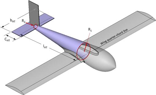
Determination of Tail Arm for a Desired VHT Such that Wetted Area is Minimized
The distance between the wings’ MGC quarter chord and the quarter chord of the horizontal tail is calculated using the following expression:
![]() (11-40)
(11-40)
Once the lHT is known, the required area, span, and average chord for the horizontal tail can be computed from:
As we have seen before, Equation (11-41) is obtained from Equation (11-37), and the two remaining ones, Equations (11-42) and (11-43), are obtained from the formulation in Section 9.2, The trapezoidal wing planform. The formulation requires a prior knowledge of the aspect ratio of the HT, but this typically ranges from 3 to 5. The reader should evaluate the ARHT for existing aircraft in the same class as the new design to use as an initial value.
Derivation of Equation (11-40)
First, we want to minimize wetted area, so let’s solve Equation (11-37) for SHT :
![]() (i)
(i)
Then, we rewrite Equation (11-39) for SWET by inserting Equation (i) into it:
![]() (ii)
(ii)
Let’s differentiate Equation (ii) with respect to lHT :
![]()
Set to zero to determine the optimum tail arm:
![]()
![]() (11-40)
(11-40)
EXAMPLE 11-5
A small airplane has a reference area SREF = 110 ft2 and a reference chord cREF = 3.5 ft. If the tail cone has the dimensions shown in Figure 11-58, determine lHT for VHT = 0.75.

Solution
Determine the optimum tail arm using Equation (11-44):
![]()
Plot the tail cone area as a function of tail arm (see Figure 11-59).
EXAMPLE 11-6
For the airplane of Example 11-5 determine lHT for VHT ranging from 0.50 to 1.00.
Solution
The solution is plotted in Figure 11-60 for horizontal tail volumes (VHT) ranging from 0.5 to 1.0. The left graph shows that as the surface area of the frustum remains constant it is the area of the HT that varies with the VHT.
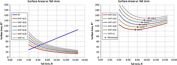
EXAMPLE 11-7
A small airplane has a reference area SREF = 130 ft2, an AR of 16, and TR of 0.5. If the tail cone has the dimensions shown in Figure 11-61, determine lHT for VHT = 0.75. Size the HT for an AR of 4 assuming a rectangular planform. Use MGC for cref.
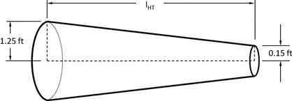
Solution
Determine the optimum tail arm using Equation (11-7):
![]()
The resulting wetted area amounts to:
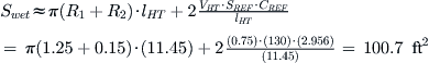
Determine tail area using Equation (11-5):
![]()
When drawn to scale, this airplane looks as shown in Figure 11-62. There is no dihedral or twist yet applied to wings, or taper to the horizontal tail, and this might represent the first “sketch” of a new aircraft.

FIGURE 11-62 A simple model based on the analysis in Section 11.5.1.
11.5.2 Method 2: Initial Tail Sizing Optimization Considering the Vertical Tail Only
This method differs from the previous one in that it shows how to size the vertical tail (rather than the horizontal tail) such that the combination of its wetted area and that of the tail arm is minimized, while ensuring the desired vertical tail volume is met. As before, the method assumes a fixed (vertical) tail volume and returns the tail arm length that results in the minimum wetted area of the design. As for the horizontal tail sizing, the method shown assumes a simplified geometry, but it can be adapted for a more complicated one.
Guidance: Note that this method does not consider the presence of the horizontal tail, only the vertical tail. It is assumed that either an alternative method will be used for the HT or it will be placed using the tail arm calculated in this section. If using this method, the designer will have to determine the size of the HT based on the tail arm calculated here. See Section 11.5.3 for a method that considers both the horizontal and vertical tail volumes simultaneously.
Assumptions
Just as before, the method assumes the fuselage aft of the wings’ quarter chord can be approximated by a frustum and the vertical tail (VT) as a constant-chord lifting surface (see Figure 11-63). If the airplane features a tapered surface rather than a constant-chord one, the quarter chord of its MGC should be placed on the quarter-chord line of the constant-chord surface. This section also develops a formulation that allows the designer to determine: (1) the required vertical tail arm (lVT); (2) vertical tail area (SVT); and (3) vertical tail span (bVT), and average chord (cVT) of the tail based on a desired vertical tail volume, VVT. In order to prepare the appropriate formulation, some fundamental geometry must be defined. For this reason, consider the dimensions of the frustum and the VT shown in Figure 11-63 and the following definitions:
![]() (11-44)
(11-44)
![]() (11-45)
(11-45)
![]() (11-46)
(11-46)
![]() (11-47)
(11-47)

Determination of Tail Arm for a Desired VVT such that Wetted Area is Minimized
The distance between the wings’ MGC quarter chord and the quarter chord of the vertical tail is calculated using the following expression:
![]() (11-48)
(11-48)
Once the lVT is known, the required area, span, and average chord for the vertical tail can be computed from:
As we have seen before, Equation (11-49) is obtained from Equation (11-45), and the two remaining ones, Equations (11-50) and (11-51), are obtained from the formulation in Chapter 7, Geometry of lifting surfaces. The formulation requires a prior knowledge of the aspect ratio of the VT, but this typically ranges from 1.5 to 2.5. The reader should evaluate the ARVT for existing aircraft in the same class as the new design to use as an initial value.
Derivation of Equation (11-48)
First, we want to minimize wetted area, so let’s solve Equation (11-45) for SVT :
Then, we rewrite Equation (11-47) for SWET by inserting Equation (i) into it:
![]() (ii)
(ii)
Let’s differentiate this with respect to lVT:
![]()
Set to zero to determine the optimum tail arm:
![]()
![]() (11-48)
(11-48)
EXAMPLE 11-8
The small airplane of Example 11-7 has a reference area SREF = 130 ft2, an AR of 16, TR of 0.5, and a tail arm of 11.45 ft. If the tail cone has the dimensions shown in Figure 11-64, determine lVT for VVT = 0.020. Select the longer tail arm of the two and size the VT for an AR of 2 assuming a rectangular planform.
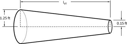
Solution
Determine the optimum tail arm using Equation (11-15):
![]()
Since lHT is larger than lVT we will us the former because this will ensure the HT has adequately long arm. For this reason, we will have to determine the tail area based on using lHT with Equation (11-13) rather than lVT:
![]()
So, we have defined the primary dimensions of the airplane in Example 11-7. The second iteration of the concept aircraft is shown in Figure 11-65.
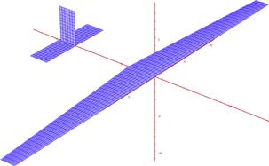
11.5.3 Method 3: Initial Tail Sizing Optimization Considering Horizontal and Vertical Tail
Many airplane configurations feature a HT and VT whose centers of lift are in close enough proximity with one another (along the longitudinal axis) to consider a simultaneous optimization for both. Figure 11-66 shows two example aircraft of many whose HT and VT can be considered close enough to optimize the tail dimensions based on both simultaneously. This section will formulate such an optimization.

FIGURE 11-66 Method 3 applies to tail feathers whose geometric centroids are pretty much equi-distance from the CG, like that of the Aeronca 7AC Champion (left). On the other hand, it is not applicable to tail surfaces arranged like that of the Aero L-39C Albatros (right). (Photos by Phil Rademacher)
Guidance: Use this method if the location of the centroids of the HT and VT are expected to be relatively close to one another along the x-axis.
Assumptions
In accordance with the previous methods, the fuselage aft of the wings’ quarter chord is approximated by a frustum and the HT and VT both as constant-chord lifting surfaces (see Figure 11-67). If the airplane features a tapered surface rather than a constant-chord one, the quarter chord of its MGC should be placed on the quarter-chord line of the constant-chord surface. The purpose of this section is to develop a formulation that allows the designer to determine: (1) the required horizontal tail arm (lT); (2) horizontal and vertical tail areas (SHT and SVT); and (3) horizontal and vertical tail span (bHT and bVT), and average chord (cHT and cVT) of the tail based on desired horizontal and vertical tail volumes, VHT and VVT. Wetted area that should be removed at the wing and tailplane junctures is not accounted for.

Formulate expressions for the SHT and SVT in terms of the tail arm LT. The planform areas of the HT and VT are defined using Equations (11-36) and (11-44).
Determination of Tail Arm for the Desired VHT and VVT
Calculate the vertical tail arm from the following expression:
![]() (11-56)
(11-56)
Once the lT is known, the required area, span, and average chord for the HT and VT can be computed from:
![]() (11-57)
(11-57)
![]() (11-58)
(11-58)
![]() (11-59)
(11-59)
![]() (11-60)
(11-60)
![]() (11-61)
(11-61)
![]() (11-62)
(11-62)
As we have seen before, Equation (11-49) is obtained from Equation (11-45), and the two remaining ones, Equations (11-50) and (11-51), are obtained from the formulation in Chapter 7, Geometry of lifting surfaces. The formulation requires a prior knowledge of the aspect ratio of the VT, but this typically ranges from 1.5 to 2.5. The reader should evaluate the ARVT for existing aircraft in the same class as the new design to use as an initial value.
Derivation of Equation (11-56)
First, we want to minimize wetted area, so let’s write Equation (11-15) explicitly for lT:
![]() (i)
(i)
Let’s differentiate Equation (i) with respect to lT:

Set to zero to determine the optimum tail arm:
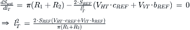
![]() (11-56)
(11-56)
QED
EXAMPLE 11-9
A small airplane has a reference area SREF = 130 ft2, an AR of 16, and TR of 0.5. If the tail cone has the dimensions shown in Figure 11-68, determine lT for VHT = 0.75 and VVT = 0.04. Size the HT for an AR of 4 and the VT for an AR of 2, assuming a rectangular planform. Here use MGC for cref.

Solution
Determine the optimum tail arm using Equation (11-56):
![]()
Determine HT area using Equation (11-57):
![]()
Determine VT area using Equation (11-58):
![]()
The resulting geometry is shown in Figure 11-69.

EXAMPLE 11-10
A small airplane is being designed with a twin tail-boom configuration (see Figure 11-70). Derive an expression for the drag optimized tail arm, similar to Equation (11-16). Use R1 and R2 to represent the base and top radii of each boom, and assume SVT to represent to total VT area.
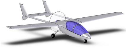
Solution
Following the same procedure we define the total wetted area as follows, noting that we have two tail-booms and not one as before:
![]() (i)
(i)
Let’s differentiate Equation (i) with respect to lT:
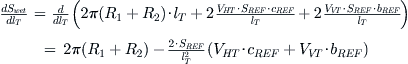
Set to zero to determine the optimum tail arm:
![]()
![]()
![]() (ii)
(ii)
Exercises
(1) The Cessna 172 Skyhawk is a very popular single-engine GA aircraft that has a reference area SREF = 174 ft2 and a wingspan of 36 ft. If its double-tapered wing has a reference TR of 0.7, determine a minimum drag LT using historical data from Table 11-4. Size the HT for an AR of 4 and the VT for an AR of 2, assuming a rectangular planform. Here use MGC for cref and assume its wing is simply tapered. Compare the resulting HT and VT to that of the original airplane. If different, explain why it differs.

References
1. Raymer Daniel. Aircraft Design: A Conceptual Approach. 4th ed. AIAA Education Series 2006.
2. NASA CR-2144. Aircraft Handling Quality Data. Heffley, Robert K., and Wayne F. Jewell Dec. 1972.
3. Nelson Robert C. Flight Stability and Automatic Control. 2nd ed. McGraw-Hill 1998.
4. NASA TM-105977. Icing Effects on Aircraft Stability and Control Determined From Flight Data - Preliminary Results. Ratvasky, T.P., and R.J. Ranaudo 1993.
5. In: http://www.historylink.org/index.cfm?DisplayPage=output.cfm&file_id=2230.
6. Cook William H. Road to the 707: The Inside Story of Designing the 707. William H. Cook 1991.
7. Abzug Malcolm J, Eugene Larrabee E. Airplane Stability and Control: A History of the Technologies that Made Aviation Possible. 2nd ed. Cambridge Aerospace Series 2002.
8. NACA TN-2175. Effect of an Unswept Wing on the Contribution of Unswept-tail Configurations to the Low-Speed Static- and Rolling-Stability Derivatives of a Midwing Airplane Model Letko. William, and Donald Riley 1950.
9. NACA RM-L54I08. Investigation at High Subsonic Speeds of the Pressure Distribution on a 45° Sweptback Vertical Tail in Sideslip with a 45° Sweptback Horizontal Tail Mounted at 50-Percent and 100-Percent Vertical Tail Span. Wiley, Harleth G., and William C. Moseley, Jr 1954.
10. NACA TR-1171. Effect of Horizontal-Tail Span and Vertical Location on the Aerodynamic Characteristics of an Unswept Tail Assembly in Sideslip. Riley, Donald R 1954.
11. In: http://en.wikipedia.org/wiki/Gloster_Javelin; In: http://www.ejection-history.org.uk/Aircraft_by_Type/Gloster_Javelin.htm; In: http://aviation-safety.net/wikibase/wiki.php?id=20519.
12. In: http://www.thevictorassociation.org.uk/?p=491.
13. In: http://aviation-safety.net/database/record.php?id=19631022-0.
14. Duffy Paul, Kandalov Andrei. Tupolev: The Man and His Aircraft. Airlife Publishing 1996; 142–143.
15. In: http://aviation-safety.net/database/record.php?id=19660603-1.
16. In: http://ntrs.nasa.gov/search.jsp.
17. NACA TN-1369. Effect of Geometric Dihedral on the Aerodynamic Characteristics of Two Isolated Vee-tail Surfaces. Schade, Robert O 1947.
18. NACA TN-1478. Wind Tunnel Investigation of the Stability and Control Characteristics of a Complete Model Equipped with a Vee Tail. Polhamus, Edward C., and Robert J. Moss 1947.
19. NACA R-823. Experimental Verification of a Simplified Vee-tail Theory and Analysis fo Available Data on Complete Model with Vee Tails. Purser, Paul E., and John P. Campell 1944.
20. NACA AC-89. Albessard Triavion Aircraft. J. Serryer 1929.
21. NASA TP-2623. Wind-Tunnel Investigation of the Flight Characteristics of a Canard General-Aviation Airplane Configuration. Satran, Dale R 1986.
22. NACA TR-1339. A Summary and Analysis of the Low-Speed Longitudinal Characteristics of Swept Wings at High Reynolds Numbers. Furlong, G. C., and J. G. McHugh 1957.
23. NACA TN-1093. Effect of Sweepback and Aspect Ratio on Longitudinal Stability Characteristics of Wings at Low Speeds. Shortal, J. A., and B. Maggin 1946.
24. NASA TM-X-26. Design Guide for Pitch-Up Evaluation and Investigation at High Subsonic Speeds of Possible Limitations due to Wing-Aspect-Ratio Variations. Spreemann, Kenneth P 1959.
1Jerzy Stanislaw Rudlicki (1893–1977) was a Polish aeronautical engineer who is considered the inventor of the V-tail. He acquired a Polish patent for it in 1930 (patent# 15938). The paper that investigated the tail is “The Rudlicki Vee Tail,” Aircraft Engineering, vol. IV, no. 37, March 1932, pp. 63–64.
2Source: www.airdisasters.co.uk/. The airplane was being operated by Northwest Airlines on October 1, 1938. The problem was solved by increasing the tail balancing – most likely that of the rudder.
3Compare that to the four-engine Tupolev Tu-114 that holds the ultimate record with a maximum speed of 473.66 KTAS (M ≈ 0.82), set on April 9, 1960, and would routinely cruise at 415 KTAS (M ≈ 0.72).