
The Anatomy of the Propeller
Abstract
A number of topics that involve the selection and performance of propellers are presented in the chapter. These range from fundamentals of propeller installation and regulatory aspects, to design and thrust generation. A section is dedicated to discussing a number of peculiar effects the propeller has on the aircraft and the aircraft designer must be aware of. Generally referred to as the P-factor, these effects include gyroscopic precession, normal and yaw force, angular momentum, as well as asymmetric thrust effects for multi-engine aircraft and A·q loads for turboprops. This is followed by a number of tips to help the designer select the right propeller, ranging from initial estimation of suitable diameter and pitch, to basics of thrust and power related coefficients, to methods helpful when selecting the number of blades. Then several procedures to estimate propeller thrust are presented. These include methods developed based on industry experience, as well as standard methods, such as the Rankine-Froude Momentum and Blade Element theories. These can be used to estimate thrust, induced airspeed in the streamtube going through the propeller, propeller efficiency, and power required to rotate the propeller.
Keywords
Propeller; tractor; pusher; nacelle; noise; propwash; fixed-pitch; constant speed; ground adjustable; two position; feathering; reversing; ground fine; beta range; helix; vortex; spinner; hub; blade; pitch angle; wind-milling; work; power; gyroscopic effects; angular momentum; slipstream; p-factor; asymmetric thrust; normal force; side force; blockage; tip effect; hub effect; A·q; loads; tip speed; diameter; efficiency; propulsive efficiency; viscous profile efficiency; Rankine-Froude momentum; blade element; compressibility
Chapter Outline
14.1.1 The Content of this Chapter
14.1.2 Propeller Configurations
14.1.5 Geometric Propeller Pitch
Pitch Angle or Geometric Pitch
Fundamental Relationships of Propeller Rotation
Determination of the Desired Pitch for Fixed-Pitch Propellers
Derivation of Equation (14-12)
14.1.7 Fixed Versus Constant-Speed Propellers
14.1.8 Propulsive or Thrust Power
14.2.1 Angular Momentum and Gyroscopic Effects
14.2.3 Propeller Normal and Side Force
14.2.5 Asymmetric Yaw Effect for a Twin-Engine Aircraft
14.2.8 Effects of High Tip Speed
14.2.9 Skewed Wake Effects – A·q Loads
14.3 Properties and Selection of the Propeller
14.3.1 Tips for Selecting a Suitable Propeller
14.3.2 Rapid Estimation of Required Prop Diameter
Derivation of Equation (14-18)
14.3.3 Rapid Estimation of Required Propeller Pitch
14.3.4 Estimation of Required Propeller Efficiency
14.3.6 Definition of Activity Factor
14.3.7 Definition of Power- and Thrust-Related Coefficients
14.3.8 Effect of Number of Blades on Power
Derivation of Equation (14-30)
Derivation of Equation (14-35)
14.3.10 Moment of Inertia of the Propeller
Derivation of Equation (14-37)
14.4 Determination of Propeller Thrust
14.4.1 Converting Piston BHP to Thrust
Derivation of Equation (14-38)
14.4.2 Propeller Thrust at Low Airspeeds
Method 1: Quadratic Interpolation
Derivation of Equation (14-40)
Method 2: Cubic Spline Method for Fixed-Pitch Propellers
Derivation of Equation (14-42)
Method 3: Cubic Spline Method for Constant-Speed Propellers
14.4.3 Step-by-step: Determining Thrust Using a Propeller Efficiency Table
Step 1: Determine Advance Ratio
Step 2: Determine Power Coefficient
Step 3: Extract Propeller Efficiency
14.4.4 Estimating Thrust From Manufacturer’s Data
14.4.5 Other Analytical Methods
14.5 Rankine-Froude Momentum Theory
14.5.4 Computer code: Estimation of Propeller Efficiency Using the Momentum Theorem
Step 4: Determine Induced Velocity
Step 5: Determine Ideal Efficiency
Step 6: Determine the Next Propeller Efficiency
Step 7: Determine the Change in Propeller Efficiency
14.6.2 Determination of αi Using the Momentum Theory
Step 3: Determine the Difference
14.6.3 Compressibility Corrections
14.6.4 Step-by-step: Prandtl’s Tip and Hub Loss Corrections
Step 1: Tip Correction Parameter
Step 3: Hub Correction Parameter
14.6.5 Computer code: Determination of the Propeller Induced Velocity
14.1 Introduction
A propeller is a device that converts mechanical energy into a force, which we call thrust, and is used to propel the vehicle to which it is attached. The propeller features one or more lifting surfaces called propeller blades1 that are rotated rapidly using an engine. The thrust is the aerodynamic2 lift force produced by the blades and is identical to the force produced by a wing. Propellers are, by far, the most common means of generating thrust for General Aviation aircraft (14 CFR Part 23). Among Light Sport Aircraft (LSA) it is practically the only means. Several types of commercial aircraft (14 CFR Part 25) also use propellers for propulsion. And a number of military aircraft do so as well; primarily trainers and several multiengine military transport aircraft. In airplanes, propellers are usually driven by piston or gas turbine engines (which are called turboprops). Additionally, electrical power is also gaining popularity (albeit mostly for light airplanes at this time), and it is converted to propulsive power using propellers.
Propellers provide a very efficient means of generating thrust by giving a relatively large mass of matter a modest acceleration (see Section 7.1.5, General theory of thrust generation). In contrast, rockets give a relatively small mass of matter a large acceleration. Generally, the larger the acceleration, the greater is the amount of chemical energy (fuel) that must be converted into mechanical energy. Thus, the generation of thrust using a propeller consumes far less fuel than any other method, making it the most efficient propulsive option currently available for airplanes. In addition, manufacturing and maintaining a propeller is far less expensive than, say, a jet engine. Therefore, propellers are really the only option for low-cost aircraft. A drawback to propellers it they are usually limited to low subsonic applications. However, the history of aviation reveals there are a number of aircraft that have been capable of relatively high subsonic airspeeds, although the cost is always considerable engine power and sophistication in propeller design.
The McDonnell XF-88B is often cited as the fastest aircraft ever equipped with a propeller. Designed in the early 1950s, the airplane was a modified prototype of the XF-88 Voodoo fighter and was actually powered by two Westinghouse J-34 turbojets. It also featured an 1800 SHP Allison T38 turboprop engine in the nose that had been installed for research purposes. The engine rotated a three bladed wide-chord propeller and was capable of high-speed flight (just exceeding Mach 1), although only thanks to the thrust generated by its jet engines. The jet version of the XF-88 later saw service with the USAF in the 1960s and became better known as the F-101 Voodoo fighter. Another aircraft, the Republic XF-84H Thunderscreech, is often called the world’s fastest true propeller aircraft.3 The aircraft was designed in the early 1950s and was equipped with a 5850 SHP Allison XT40 turboprop engine. It is claimed it achieved a speed of Mach 0.83, although this is disputed by other sources, which say it achieved only Mach 0.70. The aircraft is considered by many to have been the loudest aircraft ever built, as the outer half of the propeller blades would travel at airspeed greater than Mach 1. Allegedly, the noise could be heard 25 miles (40 km) away and was the reason for the airplane’s nickname.
The above aircraft were experimental projects that never made it to production. The fastest mass-produced propeller-powered aircraft is the four-engine Tupolev Tu-114 (Figure 14-1), which was capable of carrying over 220 passengers in a pressurized cabin at altitudes up to 39,000 ft. Its maximum speed was about 470 KTAS (M ≈ 0.82), although its cruising speed was closer to 415 KTAS (M ≈ 0.72). It featured four of the world’s most powerful turboprop engines, the Kuznetsov NK-12, each capable of developing some 14800 SHP,4 while swinging contra-rotating propellers. Although obsolete a long time ago, it was arguably way ahead of its time when designed in the mid-1950s, with its characteristic swept-back wings and lower deck galleys and deck crew rest areas. The airplane was in operation by Aeroflot from 1961 until 1976.
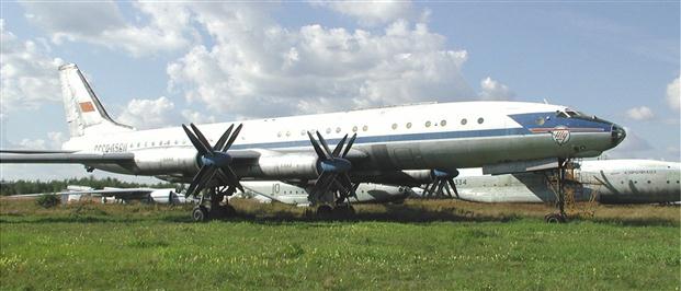
FIGURE 14-1 Tupolev Tu-114 passenger aircraft. Arguably the fastest propeller aircraft ever produced, with a cruising speed in excess of Mach 0.71. (Photo by Dmitry Avdeev – from Wikipedia Commons)
The propeller often poses serious analytical challenges for the aircraft designer. Ideally, the designer wants to determine thrust generated by a propeller using a simple variable; for instance, using the engine’s power setting. Unfortunately, reality is far more complicated. The thrust generated by the propeller is the consequence of a complex interaction between the forward motion of the propeller, its rotational speed, and geometry. This requires the designer to understand a number of fundamentals not always covered in standard undergraduate engineering university coursework. This chapter will detail two important theories that can be used to calculate propeller thrust; the Froude-Rankine momentum theory and the so-called blade-element theory. The latter, while much more complicated to use, allows the power required to rotate the propeller to be estimated. There is a third theory of propulsive thrust generation that will not be covered in this text. This is the propeller vortex theory, which, effectively, is a version of the so-called Prandtl’s lifting line theory applied to propellers. It uses potential flow theory to evaluate the flow circulation around the blades of a propeller and automatically includes the effect of the hub and propeller tip. Additionally, many authors (including the author of this book) have used the vortex-lattice method (VLM) for the same purpose, but both methods are highly mathematical and require computational proficiency well in excess of what is practical for aircraft design. These are really tools best left for propeller manufacturers to wield.
In short, the propeller is here to stay. At the time of this writing, the propeller is by far the most efficient means of turning engine power into propulsive power currently available to the designer. When it comes to efficiency, it remains superior to the jet engine. The modern turbojet and -fan have undergone substantial advances in the last 70 years, rendering it vastly superior to the turbomachinery of yesteryear. However, its efficiency is lackluster when compared to a piston engine or gas turbine that rotates a propeller. The propeller can be thought of as a bridge between design requirements and available power plants. As an example consider the 310 BHP Continental IO-550 engine. This engine is used to power aircraft ranging from the amphibious Seawind 300C, whose cruising speed is 145 KTAS, to the high-performance 185 KTAS Cirrus SR22. The dissimilarity of such aircraft shows that the interplay of mission requirements and the available power plant is bridged only by the design of the propeller. It shows the design of the propeller needs to be considered early in the design phase and should not be treated as an afterthought. Propeller design is a field of specialization requiring much more space than can be allotted here. The designer of new aircraft is well advised to establish a good working relationship with propeller manufacturers by committing to using their products early in the design process; in fact, as soon as the engine has been selected. Not only will this will lead to more accurate performance predictions, it will also reduce a number of problematic design issues that are likely to arise and lie outside the field of expertise of the aircraft designer.
14.1.1 The Content of this Chapter
• Section 14.2 discusses a number of effects the propeller has on an aircraft and which the aircraft designer must be aware of.
• Section 14.3 presents tips to help the designer select the right propeller, ranging from initial estimation of diameter and pitch.
• Section 14.4 presents methods to estimate propeller thrust.
• Section 14.5 presents the so-called Rankine-Froude momentum theory, which can be used to estimate thrust, induced airspeed in the streamtube going through the propeller, and ideal propeller efficiency.
• Section 14.6 presents the so-called blade element theory, which can be used to estimate thrust, propeller efficiency, and power required to rotate the propeller.
14.1.2 Propeller Configurations
Propellers can be mounted in a number of ways to an airplane. Three common methods are shown in Figure 14-2; a tractor (A), pusher (B), and a configuration featuring the engine and propeller mounted on the wing in nacelles (C). Configuration (C) is a variation of (A) or (B). The advantages and disadvantages of these installation methods are listed in Table 14-1. Note that so-called “inline” configurations, which consist of a tractor and pusher, can simply be treated as a combination of configurations (A) and (B).
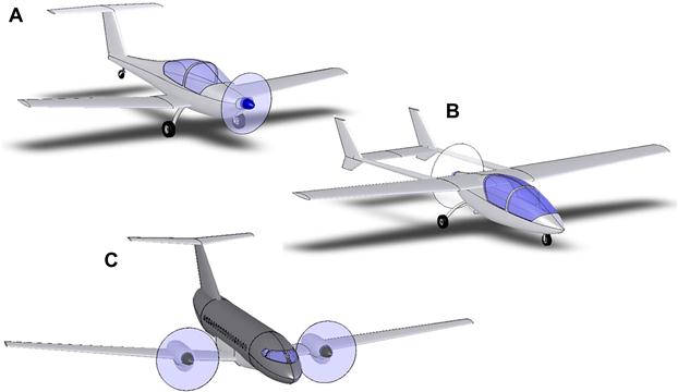
FIGURE 14-2 Three common methods to mount propellers (and engines). A is a tractor configuration, B is a pusher configuration, and C is a tractor mounted on a nacelle configuration.
TABLE 14-1
Pros and Cons of Tractor, Pusher, and Nacelle Configurations
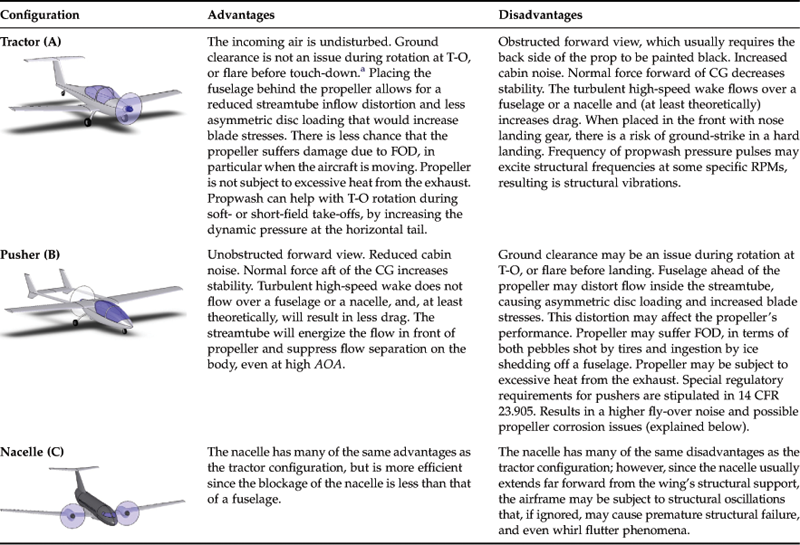
aPer 14 CFR Part 23.925 (Propeller clearance), there must be a minimum 7′′ ground clearance for a tricycle landing gear and 9 ′′ for taildraggers, at the most adverse combination of CG, weight, the most adverse pitch position of the propeller, and at static ground deflection of the landing gear. Aircraft with leaf spring struts as landing gear must comply with 1.5 times its most adverse weight.
A few additional explanations are needed for the pusher propeller. As stated in Table 14-1 special regulatory requirements affect the certification of pusher aircraft and are stipulated in 14 CFR 23.905(e) through (f). Paragraph 23.905(e) states that:
“All areas of the airplane forward of the pusher propeller that are likely to accumulate and shed ice into the propeller disc during any operating condition must be suitably protected to prevent ice formation, or it must be shown that any ice shed into the propeller disc will not create a hazardous condition.”
Paragraph 23.905(f) states that:
“Each pusher propeller must be marked so that the disc is conspicuous under normal daylight ground conditions.”
Paragraph 23.905(g) states that:
“If the engine exhaust gases are discharged into the pusher propeller disc, it must be shown by tests, or analysis supported by tests, that the propeller is capable of continuous safe operation.”
And, finally, paragraph 23.905(h) states that:
“All engine cowling, access doors, and other removable items must be designed to ensure that they will not separate from the airplane and contact the pusher propeller.”
There are further requirements made in paragraph 23.925(b) Propeller clearance that state that:
“(b) Aft-mounted propellers. In addition to the clearances specified in paragraph (a) of this section, an airplane with an aft-mounted propeller must be designed such that the propeller will not contact the runway surface when the airplane is in the maximum pitch attitude attainable during normal takeoffs and landings.”
Excluding the last paragraph, these are extra requirements not demanded by the certification of tractor aircraft. Other drawbacks of the pusher propeller that need further explanation are the higher flyover noise and propeller corrosion. Experience has demonstrated that the ingestion of fuselage wake produces additional broadband noise,5 often adding several dB(A) to the airplane’s noise. Consequently, all other things being equal, pushers tend to be noisier than tractor configurations. A pusher propeller placed behind the engine exhaust will collect soot on the blades, forming acids that attack the propeller structure. Maintenance protocols for many pushers require the operator to wash the propeller after the last flight of the day as preventive maintenance. The competent aircraft designer keeps such drawbacks in mind when choosing a pusher over a tractor. As stated in Chapter 2, Aircraft conceptual layout, there are important consequences to a configuration selection, some of which have environmental, operational, and maintenance impacts. It is not wise to base the choice on looks only – operational practicality should lead such decisions.
14.1.3 Important Nomenclature
Any discussion about propellers involves jargon that the designer must be familiar with. For instance, it is likely that in a discussion about modern aircraft, one will hear pilots and mechanics alike describing a propeller as “an advanced composite five-blade, constant-speed, reversible, and fully featherable.” What does it mean? The following definitions help clarify these terms and must be kept in mind for the discussion that follows:
A fixed-pitch propeller is a propeller whose pitch angle (the incidence of the blades with respect to the plane of rotation) cannot be changed. Such propellers are comparatively inexpensive, light, and require very little maintenance. The lack of a mechanical system renders them pretty much failsafe; however, they will windmill in the case of an engine failure and, thus, increase drag when a high glide ratio is sorely needed. Generally, such propellers are designed for best efficiency at either climb (“climb prop”) or cruise (“cruise prop”).
A ground-adjustable propeller is a propeller whose pitch angle can be adjusted using simple tools while stopped on the ground only. Thus, the operator can change the pitch from, say, a “climb” to a “cruise” style propeller (see Section 14.1.7, Fixed versus constant-speed propellers) between flights. Such propellers have become popular among homebuilders and LSA aircraft.
A two-position propeller is one that allows the pilot to change the pitch of the blades mechanically in flight, but only allows two settings (versus multiple ones for the ground-adjustable propeller). This way, the pilot could select a climb setting for the take-off and subsequent climb, and then adjust it to a coarser cruise setting once cruise altitude is reached.
A controllable-pitch propeller is one that allows the pilot to change the pitch over a range of possible pitch angles during flight. This is almost always accomplished through the use of hydraulic boost built into the hub of the propeller. Such a system allows the pilot to adjust the propeller pitch for the most efficient thrust output possible.
A constant-speed propeller is a propeller that will automatically adjust its pitch to maintain a preset RPM, which otherwise is highly affected by airspeed. It does this through the use of a controlling mechanism attached to the engine, called a governor, which balances centripetal and hydraulic forces.
A feathering propeller is a controllable-pitch or constant-speed propeller that allows the pilot to align the blades perfectly with the forward speed of the aircraft in the case of an emergency, such as an engine failure. This prevents the propeller from windmilling and, thus, reduces the drag impact of the inoperative engine.
A reversing propeller is a controllable or a constant-speed propeller that allows the pilot to align the blades to angles beyond what is possible with a feathering propeller. Effectively, it allows the thrust force to be pointed in a direction opposite to the forward motion of the aircraft. This feature is used during landing to decelerate the airplane and even to allow the aircraft to “back out” out from an air terminal using its own power. It is commonly found on turboprop engine installations.
An idealized power lever quadrant console is shown in Figure 14-3. Common reverse operation of propellers involves settings called ground fine, reverse, and beta. Ground fine is a low pitch setting used when taxiing the airplane with the engine running at a “reasonably high” rotation rate. Maintaining such RPMs on some turboprops is recommended to prevent damaging oscillation that may occur at lower RPMs. The ground fine setting prevents too high thrust from being generated at those rotation rates and this is most helpful for low-speed ground operations.
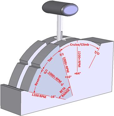
FIGURE 14-3 Idealized power lever quadrant for a typical turboprop. G/I is ground idle, F/I is flight idle, T/O is take-off.
The reverse setting, as stated earlier, generates thrust in the opposite direction and is helpful immediately after landing. The setting labeled “Taxi” in the figure is where the pilot would operate the power lever while taxiing. In this range, the RPM is constant, but the blade pitch angles are adjusted. Beta refers to the range of power lever positions that are used on the ground that include the reverse and taxi power settings.
A beta control prop is a propeller specifically designed to allow operation of the propeller as described above.
Material for propellers: the modern propeller is made from three different materials: wood, forged aluminum, or composites. All have their pros and cons, but only aluminum and composites should be used for high-performance aircraft. Wooden propellers are lighter and should not be overlooked as a solution for light airplanes that may have the CG too close to a forward limit (tractor) or aft limit (pusher).
A propeller extension can consist of a separate spacer piece (most commonly for fixed-pitch propellers) or an integral extension of the propeller hub (most common with constant-speed propellers). The purpose of the spacer or hub extension is to increase the spacing between the engine and propeller so that the geometry of the engine cover (cowling) may be made more aerodynamically efficient and, thus, reduce the drag penalty of the engine installation. This often leads to improved cooling. While heavier, the overall reduction in drag may easily surpass the penalty of the weight addition. Propeller extensions must be carefully installed because if the propeller becomes misaligned, a severe vibration may result. Ideally, it should have a centering boss to make the installation easier.
14.1.4 Propeller Geometry
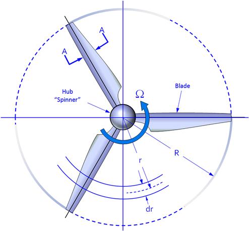
A three-bladed propeller is shown in Figure 14-4, rotating about an axis we call the axis of rotation. The spinner is an aerodynamically shaped cover, whose purpose is to reduce the drag of the hub of the propeller and to protect it from the elements. The propeller blades are what generate the thrust of the device, denoted by T. The pressure differential between the front and aft face of the propeller blade results in a vortex that is shed from the tip of the blade and is carried back by the airflow going through the propeller. This forms the typical helical shape shown in the image. Note that only one vortex is shown, but two others are also formed by the other blades and are hidden for clarity.

A frontal projection of the three-bladed propeller is shown in Figure 14-5, where R is the blade radius, r is the radius to an arbitrary blade station, and Ω is the rotation rate, typically in radians per second or minutes.
The blade of a propeller is really a cantilevered wing that moves in a circular path rather than along a straight one. Just like an airplane’s wing, the planform of the propeller blade has a profound impact on the magnitude of the thrust force created, as well as at what “cost.” What constitutes “cost” is the amount of power required to rotate it, as well as side effects such as noise. Figure 14-6 shows a picture of a typical blade planform and its cross-sectional airfoils, taken from NACA TR-339 [1]. The blade planform, along with geometric properties such as twist and airfoil camber, is of crucial importance to optimize a propeller. These affect not only the capability of the blade to generate thrust, but also its strength and natural frequencies.

FIGURE 14-6 Geometry of a typical metal propeller blade. (from Ref. [1])
14.1.5 Geometric Propeller Pitch
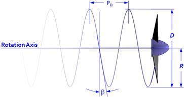
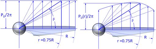
Consider the propeller in Figure 14-7, whose diameter is D and radius is R. As the propeller rotates through a full circle, its tip rotates through an arc length (circumference) of C = πD = 2πR. As the propeller rotates it “screws” itself forward a certain distance P for each full rotation. Now consider the abstract case where the propeller is assumed to rotate slowly through some highly viscous fluid. If this were possible, the propeller would move through this fluid like a metal screw moves into a piece of wood. The distance it would cover in one full revolution is called the geometric pitch or pitch distance, PD, of the propeller. It is commonly specified in terms of inches of pitch. Thus a propeller designated as a 42-inch pitch prop would move 42 inches forward in one revolution (using the metal screw through wood analogy). The angle the helix makes to the rotation plane is called the geometric pitch angle and is denoted by β.
Fundamental Formulation of
Considering the geometry shown in Figure 14-7 we can now define the following characteristics of the propeller:
where
Generally, the value of PD ranges from 60% to 85% of the diameter of the propeller. Propeller manufacturers specify the value of the pitch using the geometric pitch at 0.75R. An example of this is the Sensenich 69CK propeller used as a replacement for the Cessna 152 two-seat, single engine trainer. Its diameter is 69 inches (1.753 m) and pitch ranges from 42 to 58 inches (1.067–1.473 m).6 The pitch-to-diameter ratio is also used to identify propellers:
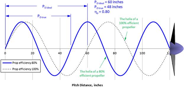
A propeller moving through a low-viscosity fluid like air will cover less distance per revolution than the geometric pitch would indicate (see Figure 14-8). Therefore, the angle formed between the rotation plane and a tangent to the blade tip helix at each blade station is less than the geometric pitch angle. This angle is called the helix angle and is denoted by ϕ. It can be estimated if the forward speed of the propeller is known using the following expression:
Pitch Angle or Geometric Pitch
Consider the cross-section A-A of the propeller blade in Figure 14-5 at some arbitrary blade station at radius r. An example of such a cross-section is the airfoil shown in Figure 14-9. In order for the propeller to generate thrust in a forward direction its chord line must form a positive angle-of-attack to the relative wind as it moves about its rotation axis. Since it simultaneously moves along the rotation axis (upward in the figure), the propeller blade airfoil must be set at a specific geometric angle with respect to the rotation plane.
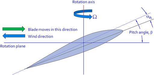
As stated before, this angle is the pitch angle or geometric pitch, here denoted by the Greek letter β (also shown in Figure 14-7). Since propeller blades usually feature cambered airfoils, their associated zero-lift AOA, αZL, is a negative number (negative AOA). Note that its reference datum is the zero-lift line of the airfoil and not the chord line. The angle between the two is αZL, as we expect from the airfoil geometric definition of Chapter 8.
Constant-Pitch Propeller
As the propeller moves in the direction of the rotation axis (i.e. in the direction of the thrust) a blade radial station near the hub experiences a relatively small airspeed component in the rotation plane, whereas the airspeed near the tip is comparatively large. The AOA experienced at a given radial station depends on this radial airspeed and the forward airspeed. Since the entire blade experiences the same forward airspeed but varying radial speed, the AOA “seen” by the airfoil at a specific radial station varies along the blade’s span. The lift generated by each radial station of an untwisted propeller would be highly uneven and, at high forward speeds, might even produce reversed thrust. Propeller manufacturers solve this by twisting the blade so that all radial stations experience the optimum AOA at some specific mission conditions, e.g. climb or cruise. This AOA is typically the one where the airfoil’s lift-to-drag ratio peaks. Therefore, the resulting propeller thrust is maximized.
The most common way of accomplishing this is to design the propeller blade such that each radial station moves a uniform pitch distance, PD, in one full turn (again, imagine it rotating in a highly viscous fluid). Since the arc length that each radial station makes varies along the propeller blade, the pitch angle closer to the hub must be at a higher pitch angle than at another one farther from the hub. Since each radial station moves a constant pitch distance, such propellers are called constant-pitch propellers (see Figure 14-10). The concept should not be confused with fixed- or variable-pitch propellers, which are discussed in Section 14.1.7, Fixed versus constant-speed propellers. Propellers designed using the constant-pitch scheme allow for a simple mathematical representation of the pitch angle β as a function of any spanwise station r, based on Equation (14-1):
where; β = pitch angle and r = arbitrary blade station along a propeller blade.
Variable-Pitch Propeller
A variable-pitch propeller is one in which the pitch distance is not fixed, but changes gradually along the span of the propeller (see Figure 14-10). The purpose of this is to load the propeller disc plane in some desirable way. For instance, it is possible the propeller designer is trying to prevent the inboard section of the propeller from stalling at some specific condition, or to prevent the section lift coefficients at the blade tip from exceeding a given maximum value at the airplane’s mission operating conditions. Or the purpose may be to modify the distribution of section lift coefficients in an attempt to make the propeller more efficient. Section lift coefficients that are too high are caused by chordwise pressure that is too low, which in turn is associated with higher airspeeds that may even exceed the speed of sound, resulting in a noisy or less efficient propeller.
Fundamental Relationships of Propeller Rotation
Consider Figure 14-11, which shows two propeller blade sections. The upper one shows the blade airfoil at a zero forward airspeed (static condition, e.g. airplane sitting on ground at rest prior to T-O). The thick vector indicates the oncoming airflow seen by an imaginary observer on the blade. The angle β is the pitch angle, whereas the AOA is represented by α as usual. The magnitude of the airspeed at that blade station in this static condition is purely dependent on the rotation rate times the spanwise distance of the blade station from the rotation axis, or:
As is evident from Figure 14-11, the AOA is the angle between the blade’s chord line and the rotation plane. Also note how the AOA changes with forward airspeed, V0, as shown in the lower portion of the figure. Note that RPM can be converted to angular velocity as follows:
![]() (14-6)
(14-6)
Additionally, we see that since the angular velocity Ω is measured in radians/second we can define the period and frequency of the rotational motion as follows:
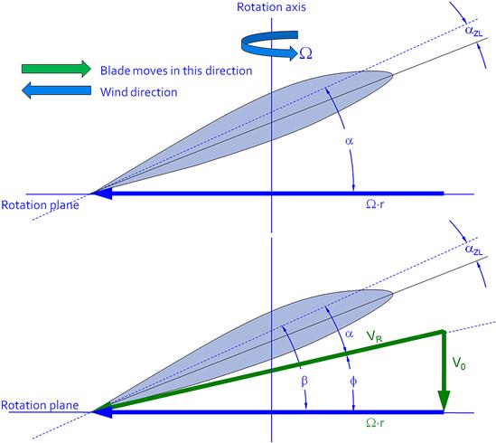
FIGURE 14-11 The upper propeller blade is rotating at static conditions (V = 0) and the lower one at some airspeed V = V0.
Now consider the lower portion of Figure 14-11, which shows the propeller as it moves at some airspeed V0 in the direction of the rotation axis. Now our imaginary observer sees the airflow coming from a different direction, at an angle ϕ, i.e. the helix angle. It can be seen that α is now much smaller than in the static case and the resultant airspeed can be obtained from the Pythagorean relation:
![]() (14-9)
(14-9)
The dynamic pressure acting on the airfoil at radial station r is based on this airspeed.
The following expressions are useful to quickly estimate the helical tip speed and Mach number of the propeller.
Determination of the Desired Pitch for Fixed-Pitch Propellers
The selection of a propeller requires its diameter and pitch to be specified. While it is recommended the designer consults with a propeller manufacturer on the appropriate dimensions, the least he can do is to be armed with a “ballpark value.” The following expression can be used to estimate the pitch of a fixed-pitch propeller whose rotation rate is denoted by RPM while operating at a desired cruising speed, denoted by VKTAS, with efficiency denoted by ηP.
Derivation of Equation (14-12)
Consider a propeller rotating at a rate indicated by RPM or RPS = RPM/60. If we assume it can operate with efficiency denoted by ηP and we know the pitch distance, PD, it follows the propeller screwing motion will move it forward at the rate shown below:
![]()
Generally, we want to refer to PD in inches and V in KTAS (and call it VKTAS). If PD is in inches it follows that V will be in inches/second. Additionally, noting that 1 KTAS = 1.688 ft/s, we introduce the following conversions:
![]()
Solving for PD leads to:
![]()
14.1.6 Windmilling Propellers
Windmilling occurs in airplanes when power to the propeller is cut and it rotates solely due to the aerodynamic lift generated by the blades. A generalized schematic of this phenomenon is shown in Figure 14-12. First consider the left image. In normal operation the prop is driven by the engine at an angular velocity of Ω and is moving at airspeed V0 through air. At a particular blade station r, the speed of the blade element is Ω·r, which yields the resulting airspeed VR and α shown. The lift, L, generated by the entire blade is shown in blue and its component parallel to the rotation axis is the thrust, T. The term w is the induced velocity, which depends on the shape of the streamtube that goes through the propeller disc.

In the right schematic, the propeller is rotating at an angular velocity Ω and some forward airspeed V0, both of which may be different from that of the left figure. This time, the speed components yield an α from the opposite side, producing lift, L, that points in the opposite direction. Again, thrust is generated, albeit in the opposite direction (and thus it should really be called drag).
Typical recovery procedures in airplanes following a non-catastrophic engine failure7 require its nose to be lowered until a specified forward speed (here denoted by V0) is achieved. This is typically the airplane’s best glide speed (see Section 19.2.8, Airspeed of minimum thrust required, VTRmin). As the angular velocity of the propeller gradually reduces, the AOA eventually becomes negative, as shown in the right image of Figure 14-12. This starts the propeller windmilling (or auto-rotating) and at this point drag begins to increase and can have detrimental effects on the L/D ratio. This effect must be considered in the aircraft design and the publication of a Pilots Operating Handbook (POH).
The reversed thrust (drag) generated by the windmilling propeller is higher than for the stationary propeller. The greater the airspeed, the greater is the propeller drag. Some pilots attempt to improve the glide ratio by stopping the autorotation. This requires the airplane to be slowed down so the propeller rotation is halted by the internal friction of the engine. More often than not this will require airspeeds in the neighborhood of the airplane’s stalling speed and, consequently, such maneuvers should not be attempted at low altitudes. Propeller-powered multiengine aircraft are always equipped with feathering propellers, which circumvent this problem by changing the pitch of the propellers such that windmilling is no longer possible and the pitch places the blades in a low-drag position, greatly reducing the impact on drag. A method to estimate the drag of windmilling (and stopped) propellers is presented in Section 15.5.13 Drag of windmilling and stopped propellers.
14.1.7 Fixed Versus Constant-Speed Propellers
Propeller efficiency is discussed in greater length in Section 14.3.9, Propulsive efficiency, but it is an indicator as to how much engine power is being converted into propulsive power (thrust × airspeed). Thus, a particular propeller may be 0.80 efficient at a specific condition. This means that 80% of the engine power (BHP) is being converted into propulsive power. As we have seen before, the AOA of the blade varies with airspeed (as shown in the lower part of Figure 14-11) and the propeller’s thrust will do so as well. It follows that propeller efficiency is a function of airspeed.
Generally, propellers for aircraft are designed for a particular airspeed or range of airspeeds specified by the airframe manufacturer. In this case the following rules of thumb apply:
For low-speed operations use a low pitch.
For high-speed operations use a large (coarse) pitch.8
A fixed-pitch propeller is one in which the blade pitch angles are permanently fixed. Such propellers are simple, light, and inexpensive. Their drawback is that their best efficiency is achieved at a particular airspeed only, so the designer must decide whether to emphasize climb or cruise performance and select a prop that favors either. Usually, two types of fixed-pitch propellers are available. The fixed-pitch “climb” propeller is designed to reach it maximum propeller efficiency at a relatively low airspeed. This makes it very suitable for use in airplanes where climb performance is of importance, such as trainers and bush-planes. The fixed-pitch “cruise” propeller is designed to reach its maximum efficiency at a higher airspeed, making it suitable for airplanes where higher cruising speed is of greater importance than climb performance.
Pilots who fly aircraft with fixed-pitch propellers notice that, if initially at cruise, the RPM of the engine will reduce if climb is initiated and increase if descent is initiated. In the former case, the climb inevitably slows down the aircraft and the propeller blades begin to experience a higher AOA. Thus they generate more drag, which, in turn, means higher torque is being generated and this slows the engine RPM. If we assume the pilot does not change the power setting, the RPM will simply drop as well and the prop will now be operating at a changed efficiency. In the latter case the opposite happens. The blades will experience lower AOA as the aircraft speeds up and generate less drag requiring less torque. The engine experiences this as reduced load so its RPM increases, again, changing the efficiency. If the aircraft is using a cruise prop, the change will be toward less efficiency, since it may very well have been operating at peak performance. If it is a climb prop, it would become more efficient as the airplane slows down, but less if it increases the airspeed.
An airplane specifically designed and operated as a cruiser will always feature a cruise-style propeller. Airspeed variations do therefore detrimentally affect its performance. This begs the question, is it possible to feature a prop that will not be so subject to such off-peak deviations? In other words: is it possible to design a prop so it tends to maintain the RPM and therefore its peak efficiency at the condition? The answer is yes. In fact, such propellers have existed for a long time and are called constant-speed propellers. However, such propellers went through an evolutionary phase, as in the 1920s manufactures, such as Pierre Levasseur, introduced manual control to adjust the blade pitch in flight [2] and that way “convert” a T-O prop into a climb prop, and a climb prop into a cruise one.
The variation in RPM with airspeed still occurred and this led to the development of an automatic controller, called a propeller governor, or simply a governor. It is designed to use accurate deviations from the setting selected by the pilot to maintain peak efficiency at all times. Figure 14-13 shows how the propeller efficiency typically varies with airspeed for three different but commercially available propeller types. The green and blue curves represent the efficiency of propellers whose pitch is fixed.

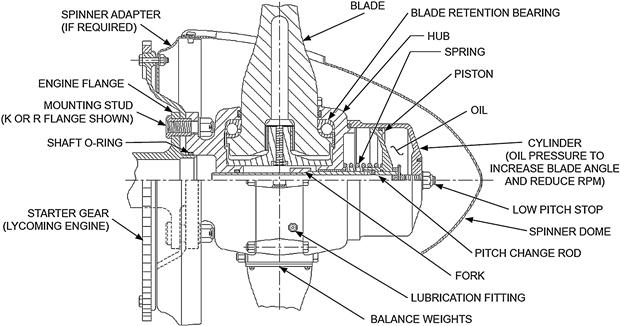
A detailed description of how the governor works is beyond the scope of this section; however, a brief introduction will be given. Once the desired RPM (using the cockpit RPM control) has been established the governor will automatically adjust the pitch of the propeller blades as needed to maintain that RPM. This is accomplished by means of throttle setting and flyweights. The governor mechanically detects RPM via the flyweights and uses it in conjunction with the throttle setting to maintain the required oil pressure inside a pressurized oil reservoir. Consider an airplane whose pitch angle deviates from a level flight such that an increase in RPM results (for instance if the nose pitches down). This implies an increase in airspeed and would cause the governor to increase the propeller pitch which would reduce the RPM. By the same token, a decrease in RPM would indicate a reduction in airspeed (for instance if the nose pitches up). The governor would then reduce the propeller pitch angle until the original RPM was again established. A section view of a hub of a constant-speed propeller is shown in Figure 14-14.
14.1.8 Propulsive or Thrust Power
Propulsive power is the power required to move a vehicle at a specific speed using specific force or thrust. Power is defined by:
![]()
Since work is defined as the application of a force over a specific distance (force × distance) we get:
![]()
We therefore define propulsive or thrust power as follows:
![]() (14-13)
(14-13)
where the subscript R stands for required as this term represents the power required in the performance analysis of later sections.
14.2 Propeller Effects
This section considers important side-effects that are caused by the presence of the propeller. These effects are so significant that the designer must be aware of them and consider them in the development of the airplane. Pilots of propeller aircraft recognize these effects, although not all understand the physics behind them, and call them the P-factor (for prop-factor). While some sources specifically call out the asymmetric yaw as the P-factor (see Section 14.2.4, Asymmetric yaw effect) others, such as Stinton [3], call the combination of the angular momentum effects (Section 14.2.1, Angular momentum and gyroscopic effects), slipstream effects (Section 14.2.2, Slipstream effects), the normal force (Section 14.2.3, Propeller normal and side force), and the asymmetric yaw effect (Section 14.2.4, Asymmetric yaw effect) the P-factor. This author agrees with this classification for the simple reason it is impossible for the pilot to distinguish between gyroscopic, slipstream, and other effects resulting from the operation of the propeller. They only feel that running the propeller at high RPM introduces effects not present when idle. In this text, the P-factor encompasses all the cited effects.
However, there are other effects to bring up that are of importance in the development of the aircraft; for instance, the asymmetric yaw effect for multiengine aircraft (Section 14.2.5, Asymmetric yaw effect for a twin-engine aircraft) that dictates which engine is critical in the case of an engine failure, blockage effects (Section 14.2.6, Blockage effects), which reduce the thrust the propeller can develop, hub and tip effects (Section 14.2.7, Hub and tip effects), the effects of high tip speed (Section 14.2.8, Effects of high tip speed), and skewed wake effects (Section 14.2.9, Skewed wake effects – A·q loads) and the resulting A·q loads that are critical for turboprops and electrically powered aircraft.
14.2.1 Angular Momentum and Gyroscopic Effects
Angular momentum and gyroscopic effects play an important role in stability and control theory and, thus, must be taken into account in the design process. Consider the propeller to the left in Figure 14-15, which rotates at a constant angular velocity Ωx (computed using Equation (14-6)). As it rotates about the x-axis (the axis of rotation), an angular momentum, hSRx, (SR stand for spinning rotor) is being generated. In conventional single-engine aircraft this momentum must be reacted by the airplane, otherwise it would itself begin to spin in the opposite direction. For instance, the angular momentum of a propeller that rotates clockwise, as seen from behind (right blade is moving down) will tend to rotate the airplane in the opposite direction – to the left. Generally, in such airplanes, this is easily suppressed by a very slight aileron deflection, since the change in lift due to aileron deflection acts through a long arm. The magnitude of the angular momentum is given by:
![]() (14-14)
(14-14)
where
(IXX)prop = moment of inertia of the propeller about its axis of rotation
Ωx = angular velocity of the propeller; the subscript x denotes rotation about the x-axis
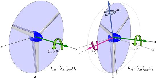
FIGURE 14-15 The left propeller rotates only along the x-axis. In the right image, it is in the process of changing orientation, which induces the restoring moments My and Mz.
Some multiengine aircraft feature an even number of engines (two, four, six, etc.) and propellers that rotate in opposite directions about the plane of symmetry. As long as the engines all rotate at the same RPM, this cancels the angular moments.
Now consider the same propeller to the right in Figure 14-15, which shows the original propeller in the process of rotating to a new orientation. This change in orientation is called gyroscopic precession. As the motion takes place, additional gyroscopic couples, My and Mz, are generated. These moments are restoring since their action is to keep the propeller in the original orientation. Note that as soon as the rotation ceases, so will those moments. If the angular velocity of the precession is given by ![]() , then the gyroscopic moments can be found from:
, then the gyroscopic moments can be found from:
 (14-15)
The components p, q, and r can be interpreted as the rotation rates of an airplane about its x-, y-, and z-axes, respectively. Note that for the propeller in Figure 14-15, the gyroscopic moments would be given by:
 (14-16)
14.2.2 Slipstream Effects
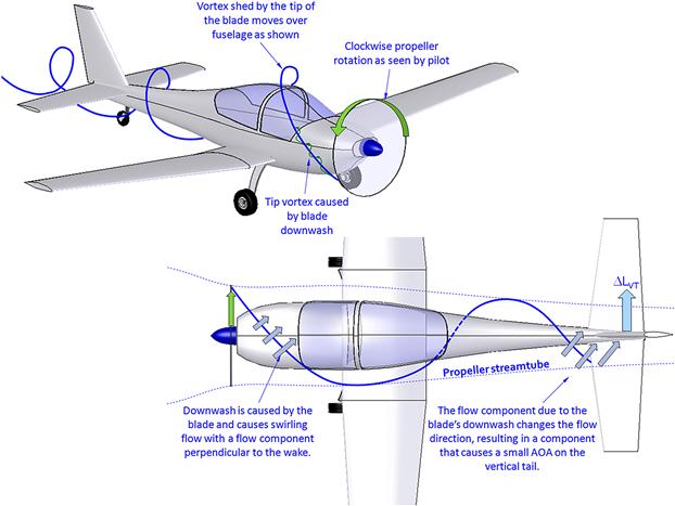
A typical single-engine aircraft is shown in Figure 14-16. It features a standard propeller whose rotation is clockwise as seen from the pilot, who sits behind it (clockwise motion of this nature is common among American propeller manufacturers, whereas counter-clockwise is common in Europe). The corkscrew-shaped blade tip vortex is sketched as it encloses the fuselage of the airplane. The tip vortex is caused by the pressure differential between the forward (low pressure) and rearward (high pressure) sides of the propeller. This pressure differential causes air on the back side of the propeller to flow toward the tip, while the opposite happens on the forward face. The opposite radial flow directions on the two sides cause the formation of this vortex at the tip, exactly as it does on a regular wing. The vortex is indicative of the downwash left by the propeller blade. The lower image of Figure 14-16 shows the vortex in the area of the vertical tail, subject to this downwash. It shows that the downwash component, which is perpendicular to the wake left by the propeller blade, changes its angle of attack, generating additional lift on it in the process. The resulting yawing moment for this aircraft (assuming a clockwise propeller rotation) tends to move the nose to the left. It can be suppressed by a rudder deflected trailing edge right (step on the right rudder), or by a cambered airfoil (camber on the left side), or by a small angle-of-incidence adjustment (leading edge left). All of these suppress the yaw by generating an opposing lift on the vertical tail. The magnitude of the yawing moment depends on engine power, RPM, and the airspeed of the aircraft.
14.2.3 Propeller Normal and Side Force
Normal Force
When an aircraft is operated at an AOA that results in the incoming flow being at an angle other than normal to the propeller disc plane, its blades will load up asymmetrically. Consider the aircraft in Figure 14-17, which shows such a condition. The lower part of the image shows the left and right halves of the propeller with an asymmetric lift distribution. This is a consequence of the right propeller blade moving in a downward motion (here, if we assume a clock-wise rotation of a two-bladed propeller, the pilot would see the right blade moving down and the left one moving up). This motion is toward an upward component of the airspeed, which, in turn, increases its lift. At the same time, the blade moving upward (the left blade) moves away from the upward component, reducing its lift. It should be kept in mind that although most of the lift of the propeller points in the forward direction, there is a vertical component to it as well. The resulting increase in lift of the right blade is larger than the reduction of the left one (due to the V2 of the dynamic pressure), causing a net force component acting in the vertical direction that adds to the normal component of the thrust. Unfortunately, the determination of the normal force is not a simple task, as it depends on the blade geometry, RPM, airspeed, and angle-of-attack of the airplane.
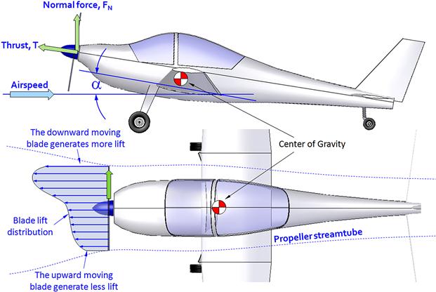
The CG of the tractor configuration in Figure 14-17 is aft of the propeller. Consequently, the normal force will destabilize the aircraft (introduce a nose pitch-up contribution). However, if the propeller is aft of the CG, as is the case for most pushers, the effect is opposite or stabilizing (nose pitch-down contribution). The moment about the vertical axis (z-axis) generated by the asymmetric disc loading also causes another effect, what pilots refer to as the “P-factor,” to be discussed next.
Side Force
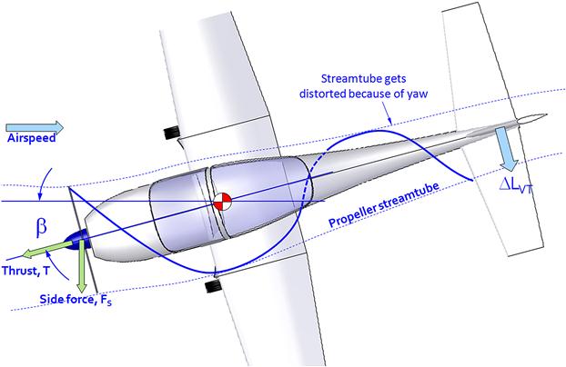
A force is generated in an identical manner to the normal force when the airplane is yawed, except it points sideways. At high power, a tractor configuration will experience a destabilizing moment (see Figure 14-18) that will tend to increase the yaw angle, requiring rudder input to correct and making it easier to exacerbate the yawed condition if care is not exercised. The designer should keep this effect in mind and ensure the directional stability (Cnβ) is large enough to prevent this from becoming a problem.
14.2.4 Asymmetric Yaw Effect
Another effect can be understood from Figure 14-17. The lower image shows the lift distribution over the propeller disc is highly asymmetric. Consequently, the right area of the disc generates more thrust than the left one. This effect generates a couple that tends to turn the nose to the left (again assuming a clockwise propeller). The pilot must step on the right rudder to suppress it. The magnitude of this couple depends on the engine power, RPM, and forward airspeed. On the other hand, the suppressing moment, which is generated by a rudder deflection, is dependent on the airspeed of the aircraft. And when the airspeed is low, the suppressing moment is low. However, the asymmetric moment may not necessarily be as low since it is highly dependent on the radial velocity of the propeller, which depends on the RPM. This highlights a potential critical flight condition for the aircraft – high power, low airspeed, high AOA, which is typical for an initial climb after take-off or during a balked landing maneuver. It is imperative the aircraft designer is aware of this effect and sizes the vertical tail to handle it.
14.2.5 Asymmetric Yaw Effect for a Twin-Engine Aircraft
The asymmetric yaw effect has serious implications for multiengine propeller aircraft. To explain this effect, consider the twin-engine aircraft shown in Figure 14-19. The left image shows the aircraft with both engines operating normally and both propellers rotating clockwise as seen from behind (note that everything said here is reversed for propellers that rotate counter-clockwise).9 As is unavoidable, both propellers are subject to asymmetric thrust loading that places the center of thrust (denoted by T) to the right of the rotation axis. The thrust of the left engine acts over a distance dL and the thrust of the right engine acts over a distance dR, which, as can be seen, is larger than dL. Therefore, a relatively small moment M is generated about the CG and this must be reacted by introducing a small rudder deflection, δr trim. For the clockwise propeller rotation shown, the moment M would result in a nose-left tendency. And while relatively small, the pilot will detect it by observing that the “ball” on the Turn and Bank indicator swings to the right of center. The pilot will respond by pressing the right rudder pedal10 or, more appropriately, by trimming the airplane nose-right using the rudder trim in an attempt to center the Turn and Bank indicator ball. Some aircraft feature a yaw-string attached in front of the windscreen and this provides the pilot with additional help by allowing him to visually assess the severity of the yaw. Note that the drag of each nacelle is denoted by DNAC, and both act over a distance dNAC.
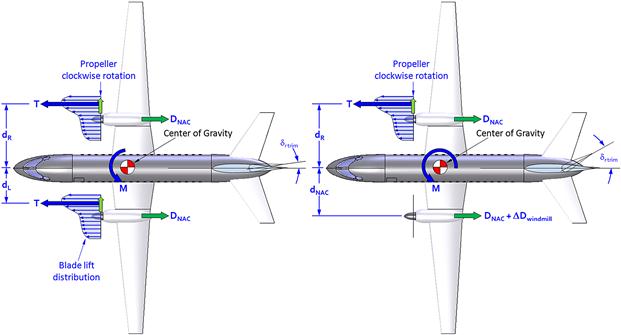
FIGURE 14-19 The consequence of asymmetric disc loading on a twin-engine aircraft in normal cruise (left) and in the case of an engine failure (right). Note that the rudder must be trimmed at a significantly higher deflection than for the normal operation, in addition to the recommended practice of “banking into the good engine” (see Figure 14-20 and text).
Now consider the right image in Figure 14-19, which shows a scenario in which the left (critical) engine has failed. This situation is referred to as flying with one engine inoperative (OEI) and can present a very serious situation to the pilot. An inspection of Figure 14-19 shows that a failure of the left engine results in a substantially greater moment than if the right engine fails. For this reason, the left engine is called the critical engine. In other words, an inoperative left engine presents a greater problem to the pilot than a failed right engine. The asymmetric thrust will cause a powerful moment, M, that forces the aircraft to yaw toward the dead engine. This may be compounded by the fact that the propeller may now be windmilling with the associated increase in drag (ΔDwindmill) of the dead engine. The drag may be reduced by feathering the propeller (see Section 14.1.3, Important nomenclature), which is a mechanical feature offered on most twin-engine aircraft.
The standard procedure in this situation is for the pilot to eliminate the yaw by stepping on the rudder pedal on the same side as the functional engine. This is followed by banking the airplane between 2° and 5° toward the functional engine (see Figure 14-20). Once this has been established, the pilot will “feather” the dead engine.

FIGURE 14-20 The standard practice of “banking into the good engine” is used to reduce required rudder deflection when flying with one engine inoperative. However, when slowing down for landing it becomes harder and harder to maintain altitude in the configuration.
Let’s consider these actions in more detail. Pilots are trained to identify which side the dead engine is by stepping on the rudder pedals. It takes considerably less force to press the pedal on the same side as the dead engine compared to the one on the side of the functional engine.11 This is caused by the floating tendency of the rudder, but without control inputs the condition causes the airplane to yaw (and bank) toward the dead engine. For the aircraft of Figure 14-19, before the pilots makes corrective control inputs, it will yaw so its right side is windward. The rudder will thus float trailing edge left and this is why the left rudder pedal feels dead.
Banking toward the functional engine establishes a turning tendency that reduces the rudder deflection required to maintain heading. Increasing banking may even eliminate the need for rudder input, but usually at the cost of the already impaired performance. There is a limit to how much banking should be applied. If the bank angle is too great the rate-of-climb could easily be detrimentally affected and could prevent the aircraft from maintaining altitude. As a rule of thumb, in order to achieve the maximum rate-of-climb in the OEI configuration (VYSE) a bank angle of 2° is recommended if the non-critical engine fails, and 3° if the critical engine fails. A bank angle in excess of 5° almost certainly results in rate-of-descent (loss of altitude) for underpowered twins.
Another situation may confront the pilot operating a twin in an OEI configuration. If the airplane is slowed down below a certain airspeed, control authority will be lost and the rudder will be incapable of opposing the yaw. This airspeed is called minimum control airspeed, denoted by VMC. If the airspeed falls below this airspeed, the aircraft will roll upside down, possibly causing an inverted spin, if not impacting the ground first. At any rate, it is a likely fatal scenario for all the occupants. For this reason it is imperative the pilot maintains high enough airspeed at all times, and slows down only after reducing power and pointing the nose down. The minimum control airspeed (VMC) is usually higher than the airplane’s stalling speed (VS) and rotating to take-off should not be performed until after it is reached and exceeded.
This scenario is remedied by installing a right engine/propeller combination that rotates counter-clockwise (or opposite to that of the left engine). Figure 14-21 shows such a configuration. Interestingly, an examination of aviation history reveals this is in fact rarely done. This is called a counter-rotating configuration.12 Albeit safer, the primary drawback of that configuration is that it is more expensive to produce, as logistically it must feature two engines and propellers that are dissimilar because they rotate in opposite directions. An operation of such an aircraft results in greater expenses as engine parts are no longer interchangeable. This can pose a peculiar situation for an operator, which might have parts for the left engine on hand, while none are in stock for a failed right engine. Such scenarios should not be overlooked when selecting an engine configuration as this could severely impact the finances of an operator. Instead, the designer should size the control system and surfaces to handle the critical engine. For this reason it is imperative the aircraft designer is fully aware of this condition.
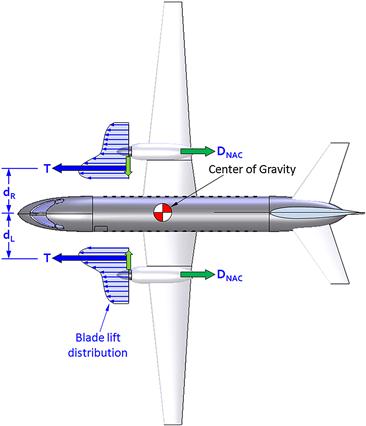
FIGURE 14-21 An aircraft with counter-rotating propellers as shown here does not have a critical engine and is a safer design, albeit operationally more expensive.
It is of interest to note that the Wright Flyer featured two counter-rotating propellers, although this was due to the nature of the single engine drive train. It is almost certain that the notion of asymmetric thrust would not have entered the minds of the pioneers of aviation at the time. Among other aircraft that feature this option are the De Havilland DH-103 Hornet, which was a derivative of the DH-98 Mosquito. The Lockheed P-38 Lightning featured counter-rotating propellers, although, surprisingly, both propellers rotated inversely of what is shown in Figure 14-21. This suggests that a cancellation of propeller torque was driving that design decision and not asymmetric yaw. An identical arrangement is found on the Heinkel He-177 Greif. Among other aircraft is a series of Piper aircraft, in order of models, the Piper PA-31 Navajo Chieftain, PA-34 Seneca, PA-39 Twin Commanche, the cancelled PA-40 Arapaho, and the PA-44 Seminole. Other aircraft include the Cessna T303 Crusader, Beech Model 76 Duchess, and Diamond DA-42 Twinstar, all of which feature counter-rotating piston engines. All of these are designed with the correct propeller rotation shown in Figure 14-21.
It is interesting to note that large airplanes typically don’t feature propellers that rotate in opposite direction. Even large aircraft, such as the four-engine Lockheed P-3C Orion and C-130 Hercules, feature propellers that all rotate in a clockwise direction. This is an example of a design decision that focuses on reducing maintenance costs in lieu of safety. Of course, for the above aircraft, an easy counter-argument is to be made that safety is in fact not compromised, but maintained by requiring rigorous pilot training, as well as providing hydraulically actuated control surfaces, and very powerful engines – an argument that is hard to dispute. Many larger aircraft provide a rudder boost system; a pneumatically powered actuators that force the rudder to the proper deflection angle to counter the asymmetry [4]. Such systems detect which engine has failed and react accordingly – providing substantial safety to the operation of the aircraft. In addition, the operational history of these aircraft supports this notion – there are not many accidents in current times that can be attributed to asymmetric thrust on larger propeller-powered aircraft. However, for small twins this is not the case, as will now be demonstrated.
It is of great importance that the designer understands the implications of selecting a twin-engine configuration, in particular if the engine power is relatively low. In addition to increased acquisition and maintenance cost, the selection has important safety and performance implications associated with it. From a development standpoint, such configurations generate more drag than a single-engine aircraft of the same power (assuming a conventional on-wing engine layout). This results from the presence of two nacelles on the wing in addition to the fuselage. This impact on drag can be reduced by a twin-engine configuration such as that of the Cessna 337 Skymaster and Adam A500 aircraft. However, what is more serious is the performance degradation that results if one engine fails. If a spacious cabin and high cruising speed are desired, a solution such as is offered by recent small GA aircraft should be considered. Aircraft such as the French SOCATA TBM-700 and TBM-850 and the Swiss Pilatus PC-12 are powered by a single Pratt & Whitney PT-6 turbine engine and are capable of cruising speeds in excess of 300 KTAS at 30,000 ft. This beats any of the above twin-engine piston aircraft (excluding the P-38).
To discuss the effect of engine power on the performance of a generic twin-engine piston aircraft consider Figure 14-22. The aircraft portrayed is in the small Piper Apache size class of aircraft. The figure shows that in normal operation, the aircraft climbs 1478 fpm at S-L and offers a maximum speed of 173 KCAS. Upon losing an engine the best rate of climb will drop to 239 fpm and its maximum speed to 97 KCAS. The analysis assumes a drag degradation associated with maintaining a straight heading with OEI by adding 50 drag counts (ΔCD OEI) to the original minimum drag. This is reasonable based on the airplane being flown cross-controlled in a yawed configuration. The problem with this turn of events is that the low rate of climb does not allow a lot of room for mistakes. In light of the low-power sensitivity, an inexperienced or frantic pilot may easily maneuver the airplane off the peak conditions, causing it to lose altitude.

14.2.6 Blockage Effects
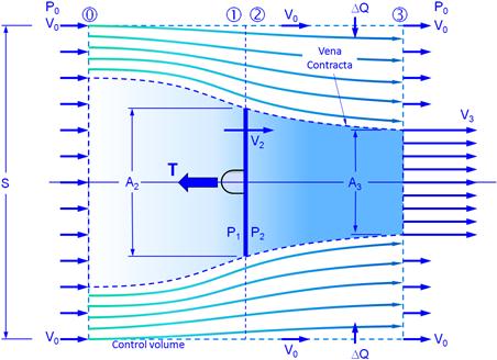
There are two kinds of blockage effect. First is a body placed in the streamtube ahead of the propeller disc (a pusher configuration). The other is a body placed in the streamtube behind the disc (tractor configuration). An idealized streamtube going through a propeller disc is shown in Figure 14-46. Placing an obstruction such as a fuselage (or a nacelle) into the streamtube will distort it and prevent the formation of a proper vena contracta. This will reduce the acceleration of the flow in the streamtube and, thus, the resulting thrust. Figure 14-23 shows an ideal (“Unblocked”) streamtube superimposed on what the actual (“Blocked”) streamtube might look like.
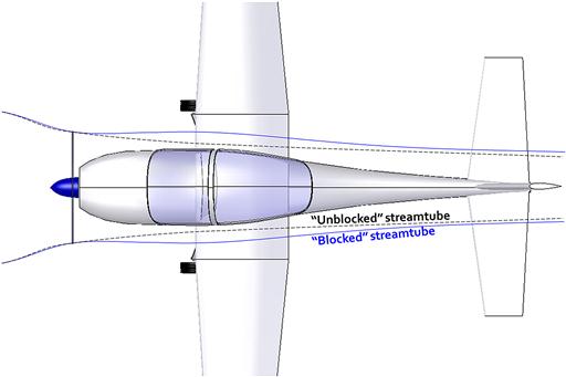
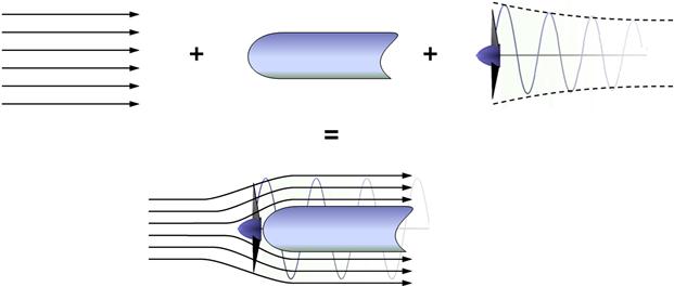
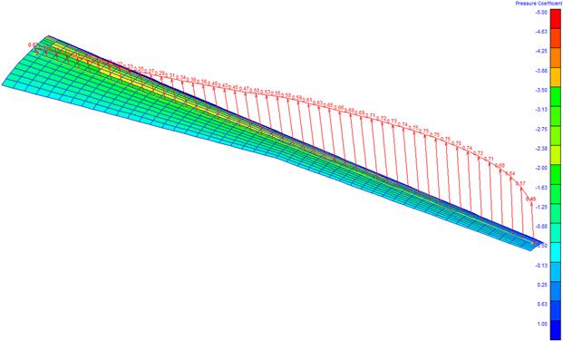
FIGURE 14-25 Section lift coefficients for a propeller blade of a small wind turbine, showing reduction in lift coefficient near the root (left) and the tip (right).

FIGURE 14-26 A flight condition (climb) that generates a skewed wake (upper image) and the definition of the inflow angle A (lower image).
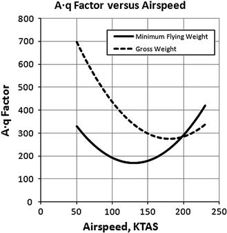
FIGURE 14-27 Skewed wakes at extreme weights reveal two distinct minimums – a compromise between the two should be made.

FIGURE 14-29 A graph from www.faa.gov showing the current noise level limitations for propeller aircraft (G36.301 Aircraft noise limits).
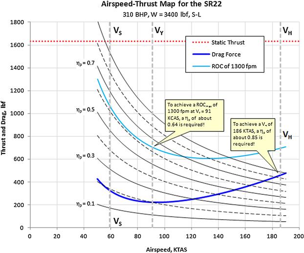
FIGURE 14-30 An airspeed-thrust map shows the propeller efficiency required to meet given performance characteristics in terms of thrust.

FIGURE 14-31 An airspeed-power map shows the propeller efficiency required to meet given performance characteristics in terms of power.

FIGURE 14-32 Influence of airspeed (left) and blade area ratio (right) on the size of a three- and four-bladed propellers intended to replace a two-bladed one.
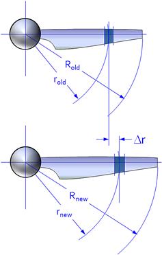
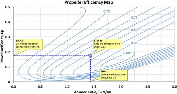
FIGURE 14-34 An idealized propeller efficiency map. Such maps are always drawn for a specific propeller activity factor. Note the island where ηp = 0.88 is where the propeller should be sized to operate.
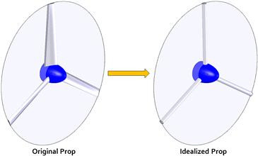
FIGURE 14-35 Idealizing the prop as constant-diameter rods allows for a fast estimation of its moment of inertia.
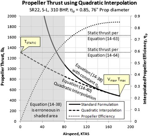


FIGURE 14-38 As the Piper J-3 Cub accelerates from rest to VH, it moves through the isobars as shown.

FIGURE 14-39 Plotting T(VKTAS) at full power and S-L for the Piper J-3 Cub with a fixed-pitch propeller.
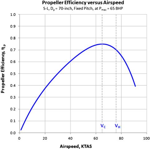
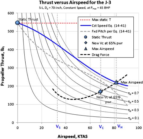
FIGURE 14-41 Plotting T(VKTAS) at full power and S-L for the Piper J-3 Cub with a constant-speed propeller.
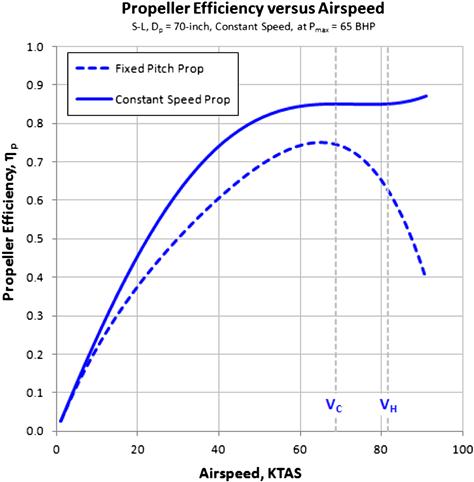
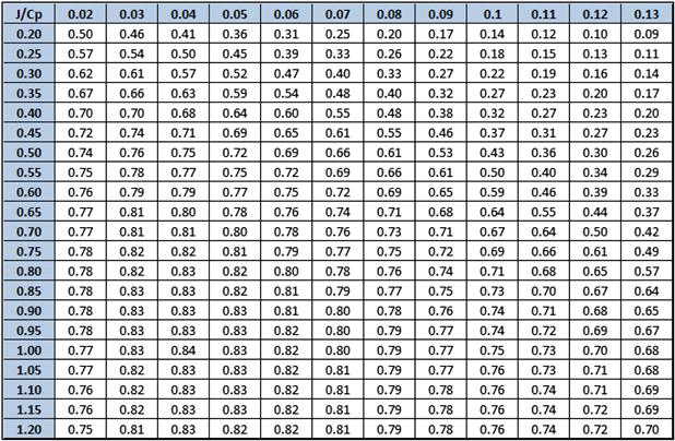
FIGURE 14-43 A typical propeller efficiency table for a constant-speed propeller (no specific propeller type).

FIGURE 14-45 A typical propeller efficiency graph for a fixed-pitch propeller (no specific propeller type).
An estimation of the impact of blockage effects requires the flow around the obstruction to be incorporated into the wake model (for instance, see the wake of Section 14.5, Rankine-Froude momentum theory). The most reliable approach (excluding empirical methods) is to use the method of superposition depicted in Figure 14-24. A version of this approach is detailed in NACA TM-492, Influence of Fuselage on Propeller Design, and NASA CR-4199, An Analysis for High Speed Propeller-Nacelle Aerodynamic Performance Prediction. The mathematics of these methods are beyond the scope of this book. The manufacturers of propellers do consider blockage effects in the design of their propellers, although the methods used are usually proprietary. The aircraft designer can help mitigate blockage problems by considering a hub extension for piston-engine aircraft and select the largest spinner possible to cover the inboard and least efficient portion of the blade. This allows the cowling or nacelle to be sculpted in a manner that provides less obstruction to the flow. Ideally, the cowling or nacelle should be designed to be as axi-symmetric as possible, as this will yield higher installed propeller efficiency.
14.2.7 Hub and Tip Effects
The presence of the hub (root) and the tip of the blade will have a large effect on the distribution of section lift coefficients, as this is where lift must necessarily go to zero. The blade of a wind-turbine is shown in Figure 14-25 (hub is omitted from the view), and shows how the lift diminishes near the root (left) and tip (right). The effect is less noticeable near the root, because the radial speed of the air is less there. However, the tip shows how the section lift coefficients drop rapidly. Naturally, the twist of the blade and camber of the airfoil will influence this as well, but the figure illustrates that the phenomenon will affect thrust. For this reason, hub and tip effects must be taken into account when analyzing the thrust of the propeller. The so-called Prandtl’s tip and hub loss correction is presented in Section 14.6.4, Step-by-step: Prandtl’s tip and hub loss corrections, where it is used to correct analysis made by the blade element method. The correction method uses the geometric features of the propeller to approximate the reduction of the section lift coefficients and is relatively simple to apply.
14.2.8 Effects of High Tip Speed
The primary effect of a high tip speed is the risk of the formation of shock waves on the blade, which leads to a reduction in the propeller efficiency, increase in torque (requires more power to turn it), and an increase in the noise emitted by the propeller. The pitch, thickness, and curvature of the blade airfoil accelerate air well beyond what the tip speed might indicate. These effects are best avoided by selecting rotational tip speeds in the M ≈ 0.6 range for wooden propellers and in the M ≈ 0.75–0.8 range for metal and composite propellers.
14.2.9 Skewed Wake Effects – A·q Loads
A skewed wake is one for which the streamtube inflow through the propeller disc is not normal to its plane (see Figure 14-26). Such a wake is encountered any time a propeller-powered aircraft climbs or yaws. In general, there is no significant effect on the propeller performance, and usually the effect is most severe during transient maneuvers. However, the skewed wake has important effects on noise and propeller loads, especially for turboprops. Let’s consider these effects in some detail.
Consider the airplane in Figure 14-26, which presents a condition in which the propeller thrust line is not aligned with the flight path. Consequently, the streamtube is at an angle A to the thrust line (or normal to the propeller disc plane). As the propeller rotates at an angular speed Ω, each down-turning blade will encounter an increase in its AOA and each up-turning blade will see a reduction in its AOA, as explained in the discussion about the normal force. This will load up each blade and subject it to cyclic loading at the frequency described by Equation (14-8). This is commonly referred to as 1P cyclic loading, where 1P stands for once per revolution. A byproduct of this is increased noise.
As stated above, the phenomena increases the propeller’s 1P loads, which is the main source of loads for a turboprop. These loads are directly proportional to the product of the angle A and the dynamic pressure of the free-stream, q. For this reason they are often referred to as “A·q” loads. For piston-propeller configurations, the primary load of the propeller is caused by the sudden acceleration resulting from the shock of the cylinders firing and the subsequent torsional deformation of the crankshaft. These loads are much greater than the A·q loads.
However, for turboprops (and for electric aircraft) the A·q loads are critical. For this reason, it is imperative the designer of turboprop and electric aircraft performs careful mission performance analyses to determine the AOA of the vehicle at a representative cruise condition and then align the thrustline so it is mostly parallel to the flight path (the inflow angle A = 0°). Clearly, this cannot be achieved over the entire airspeed range, so propeller manufacturers recommend a “balanced” approach. That is, the product A·q is determined at the maximum and minimum operating weights (see Figure 14-27). Then, the thrustline is aligned for zero inflow angle between the two minimums, guaranteeing the least A·q loads possible. Of course low load is desirable: the less the load, the lighter the propeller. Failure to follow these guidelines may result in the design failing article 14 CFR 23.907 Propeller vibration and fatigue, which may cause a major redesign effort, with the associated development costs and program delays.
14.2.10 Propeller Noise
Noise associated with the operation of aircraft remains a topic of (often) hotly contested debate in society. One consequence of this debate has been a substantial reduction in aircraft noise over the last 25 years or so, in particular for jet aircraft. This has been achieved by a combination of new regulatory policies and increased research effort. Noise pollution generated by propellers has also been brought to more tolerable levels, although many aircraft types, primarily high-performance piston aircraft, still feature engines that operate at high RPMs at full power, resulting in objectionable noise pollution. Like all other aspects of aircraft design, noise level is a tradeoff with cost, weight, performance and other parameters. What remains is that noise pollution from propellers can be significant and should be seriously considered by the designer from the start of the design project. It is best to work with a propeller manufacturer and use their expertise to design and select propellers that are both quiet and efficient. Current manufacturers of propellers have responded with propeller blade designs that feature airfoils of lower thickness-to-chord ratio and swept planform geometry near the tip. An example of such a design is the scimitar-shaped propeller in Figure 14-28. Such blades are intended to reduce the magnitude of low-pressure peaks and delay the onset of normal shocks that increases the noise. Additionally, the trend has been toward an increased number of blades, as this allows the propeller diameter to be reduced, which, in turn, reduces the tip airspeed. Engine operating RPMs have also been reduced.
Propeller aircraft must comply with the requirements of 14 CFR Part 36 Appendix G [5]. Among a number of stipulations, this requires the aircraft to fly over a microphone placed some 8200 ft (2500 m) from brake release and the noise to be measured. The measured noise level must not exceed that shown in Figure 14-29.
The aircraft designer should not forget that two aircraft that use exactly the same engine and propeller combination can have two different measured noise levels. All other things being equal, the aircraft with the larger wing area and wing span will lift off using a shorter ground run, and it will climb faster at a lower airspeed (VY; see Chapter 14, Performance - climb), resulting in a steeper climb gradient. In short, it will climb to a higher altitude in the given distance of 8200 ft, resulting in a lower measured noise level. If there is a concern the aircraft may not or marginally comply with 14 CFR Part 36, the designer should perform a sensitivity study of wing geometry and noise levels.
Reference [6] presents a simple method to theoretically predict the near-field and far-field noise of propellers.
14.3 Properties and Selection of the Propeller
A number of issues must be considered during the selection of a propeller for a new aircraft design. The designer should consult the propeller manufacturer early on to help with the selection. Usually this process involves the designer providing the propeller manufacturer with detailed information about the new (or modified) aircraft. The propeller manufacturers generally have some form of design specification that the aircraft designer can complete to efficiently transmit all of the relevant information to the propeller manufacturer. This information is used by the propeller manufacturer to select an existing design, or in some cases a new blade design is warranted.
14.3.1 Tips for Selecting a Suitable Propeller
Although the aircraft designer should benefit from the experience of the propeller manufacturer, he should also be armed with a number of parameters. Among those are:
(1) An estimate of the propeller diameter. Section 14.3.2, Rapid estimation of required prop diameter, provides methods that help estimate the diameter of several types of propellers.
(2) An estimate of the propeller pitch. Section 14.3.3, Rapid estimation of required propeller pitch, provides methods that help estimate the required pitch for a fixed-pitch propeller.
(3) The airplane’s target performance: requirements for take-off and climb performance, mission cruising speed and altitude strongly affect the selection of the propeller type. Are these best met using a constant-speed propeller, or will a fixed-pitch design do? Traditionally, if the engine power is greater than 180–200 BHP, and the cruising speed is in excess of 130–140 KTAS, a constant-speed propeller is recommended.
(4) Engine characteristics, such as the rated BHP, operational RPM, and torsional vibration play an important role in the selection of the propeller diameter and number of blades. The installation of the engine on the airframe may cause detrimental interferences between components of the airplane and the propeller blades. The shape of the nacelle influences the installation as well and sometimes requires a hub extension so that a more aerodynamically “friendly” external geometry can be designed. Additionally, the presence of a body in front or behind the propeller distorts the flow in the streamtube going through the propeller and will affect its efficiency. Therefore, the entire configuration of the aircraft must be considered. Is the propeller for a single or a multiengine aircraft? Shall it rotate clockwise or counter-clockwise? It is a tractor or a pusher? Moreover, a number of systems are required to operate the propeller. For instance, a de-ice system may be required for flight into known icing, a propeller pitch control, and possibly a gear-reduction drive. And finally, there is always a concern for cost, weight, noise, and efficiency. In the addition to the above, the selection process should also consider the following considerations:
• Tip (refers to rotational and not helical) speed should be as high as possible, but there is an upper limit. Too high a tip speed increases noise and reduces efficiency (via shock formation).
• Rotational tip speeds for wooden propellers13 are in the M ≈ 0.6 range.
• Rotational tip speeds for metal propellers14 are in the M ≈ 0.75–0.8 range.
• Rotational tip speeds for advance composite15 propellers are in the M ≈ 0.75–0.8 range.
• If the engine RPM is too high a gear-reduction drive may be required to slow it down.
• High rotational speed requires fewer blades or a smaller blade area to generate thrust.
• High-powered engines whose rotational rate limits the propeller radius need more blades to help convert engine power into thrust.
• Too large a diameter may result in high tip speeds and noise, but can also present some ground proximity problems.
• Weight – a three-bladed prop can be of a smaller diameter, but three blades weigh more than two blades.
When considering thrust per number of blades, the fewer the blades the more efficient is the propeller. However, this should not be taken to mean that a prop with a large number of blades can’t have propeller efficiency equal to or higher than a comparable two-bladed propeller.
14.3.2 Rapid Estimation of Required Prop Diameter
The conceptual design of propeller-powered aircraft often requires the prop diameter to be quickly estimated. This is crucial in determining various characteristics, ranging from thrust for performance analysis to propeller noise and geometric constraints, such as the likelihood of a ground-strike. This section considers a couple of such rapid estimation methods. Stinton [3] presents a method to calculate the diameter of wooden propellers in inches, based on the intended cruising speed in KTAS, engine power, and RPM.
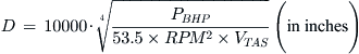
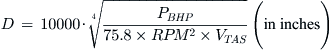
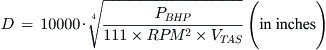
Derivation of Equation (14-18)
The source document does not derive Equations (14-17) or (14-19), but states that values for a three-bladed propeller can be obtained by interpolating between the two expressions. This leads to the following closed-form equation for the closed three-bladed propeller:
![]()
Manipulating algebraically leads to:
![]()

QED
EXAMPLE 14-2
The Aerotrek A240 Light-Sport Aircraft is equipped with a 62.2 inch diameter three-bladed composite propeller. When powered by an 80 BHP Rotax 912UL engine it is capable of flying at 104 KTAS at 75% power. Calculate the recommended diameter of two-, three-, and four-bladed wooden propellers for this airplane, intended to rotate at 2300 RPM, and compare to the actual propeller diameter. What are the corresponding tip speeds?
The same source states that the diameter of three-bladed metal propellers in inches can be obtained from the following expressions.
Raymer [7] presents the following expression, independent of propeller material, which he states are modified from those of Stinton. The corresponding propeller diameter in ft or meters depending on Kp:
where the factor Kp is obtained from Table 14-2.
14.3.3 Rapid Estimation of Required Propeller Pitch
For a fixed-pitched propeller, the required pitch can be determined from Tables 14-3, 14-4, and 14-5. The first table represents the ideal, but physically impossible propeller with an efficiency of 100%, while the other two show pitch for 90% and 80% efficient respectively. The table is assembled using Equation (14-12) and is read as shown by the shaded cells. A 100% efficient propeller rotating at 2700 RPM must feature a 56 inch pitch in order to achieve 120 KTAS. The tables are intended to give the designer an idea of the propeller pitch required.
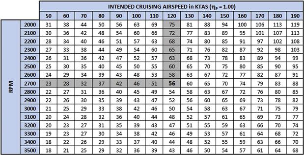
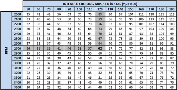

14.3.4 Estimation of Required Propeller Efficiency
Once a trustworthy drag model of an aircraft has been prepared, it is appropriate to evaluate the type of propeller that will be required based on its required propeller efficiency. This section shows how to do this in an effective manner. This involves the preparation of airspeed-thrust (see Figure 14-30) or airspeed-power (see Figure 14-31) maps. It does not matter which one is prepared, as long as one of them is. The maps show thrust and power in terms of propeller efficiency isobars. Then, important desirable performance characteristics can be added on a need-to basis. The map shows at a glance the propeller efficiency required to achieve those characteristics. It is easiest to explain such maps using an example. Here the SR22 is the obvious choice.
First consider Figure 14-30. The isobars are plotted using Equation (14-38) for constant values of ηp. The static thrust was calculated using Equation (14-63). Then the drag force is plotted based on the available drag model. The drag model for the SR22 was extracted using POH data in Example 15-18. It is then used to plot the drag force curve shown in the graph. The ROC curve is based on solving Equation (18-17) for thrust required to achieve a given ROC:
![]()
Here 1300 fpm was selected, as this is close to the capability of the SR22 at gross weight at S-L at V = 91 KCAS (recall that at S-L KCAS and KTAS are equal). This way, it is possible to explore the capability of its propeller. The graph of Figure 14-30 shows that a prop efficiency of around 0.85 is required to achieve a top speed of 186 KTAS at S-L. Similarly, in order to achieve the ROC at VY, the prop efficiency must be around 0.64. This sort of information can be very useful to the propeller manufacturer when helping to select or design a practical propeller.
Figure 14-31 is identical to Figure 14-30, except it uses power rather than force to relay the same information. Therefore, the propeller efficiency isobars are horizontal lines, which may make it a tad easier to evaluate the propeller efficiencies. Other than that, it gives exactly the same answers as the airspeed-thrust map.
14.3.5 Advance Ratio
The advance ratio is a measure of how far the propeller travels in unit time in terms of its diameter. The distance the prop travels per second is the vehicle’s speed through the medium and is given by V0. For instance, if we measure an advance ratio of 0.5 for a 10 ft diameter propeller rotating at 600 RPM it means the propeller (i.e. the vehicle it is propelling) is moving at a forward speed of 50 ft/s.
EXAMPLE 14-3
The SR22 is equipped with a 76 inch diameter propeller. If the airplane is observed to fly at 185 KTAS at 8000 ft with the propeller rotating at 2700 RPM, what are the helix angle, blade rotational and helical tip speeds, Mach number, and advance ratio?
14.3.6 Definition of Activity Factor
The activity factor (AF) represents the power absorption capability of all blade elements. Small aircraft have an AF ranging from 80-105, while larger aircraft have an AF around 130-170. The AF is used when reading propeller efficiency maps, which are special contour maps prepared by the propeller manufacturer that allow propeller efficiency to be read as a function of the advance ratio and power coefficient (see Section 14.3.7, Definition of power- and thrust-related coefficients):
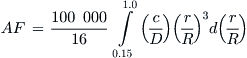
where
See the list of variables at the end of this chapter for other variable details.
EXAMPLE 14-4
What is the activity factor of each blade of the airplane of Example 14-3, whose diameter is 76 inches and chord is a constant 5 inches.
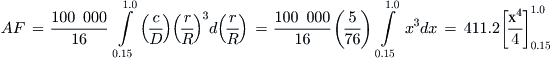
14.3.7 Definition of Power- and Thrust-Related Coefficients
The following concepts are definitions:
By combining Equations (14-26) and (14-28) we get:
See the list of variables at the end of this chapter for variable details.
EXAMPLE 14-5
Compute CP and CQ for the airplane in Example 14-3 for the same condition, if it is known its engine is generating 225 BHP.

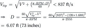
14.3.8 Effect of Number of Blades on Power
The number of blades is fundamental to how the engine power is converted into propulsive power. Replacing propellers is a common occurrence in the aviation industry. Sometimes such changes involve a propeller that has a different number of blades than the original prop. For instance, consider a four-bladed propeller as a replacement for a two-bladed one. Assuming such a modification only involves a change in the number of blades, the addition will increase the torque required to swing the new propeller by a factor of two. This can be seen, for instance, in the formulation developed in Section 14.6, Blade element theory. However, since this propeller will be mounted on the same engine, the power available per blade will diminish. This will manifest itself in the engine being unable to rotate the propeller at the original RPM. With everything else being equal (e.g. propeller diameter and blade planform geometry being the same) less thrust will be generated and the performance of the airplane will suffer. The remedy is to reduce the torque generated per blade, as this will allow the propeller to be rotated at RPM closer to the original one. The easiest way to accomplish this is to reduce the diameter of the propeller. An advantage of such a modification is less propeller noise and weight. Also, the ground clearance of the prop will increase (assuming the number of blades is increased), rendering this an important option at the discretion of the designer struggling with potential prop strike issues.
It is of interest to estimate what propeller diameter is appropriate when changing the number of blades, regardless of whether the intent is to increase or reduce the number of blades. This can be done by solving the following expression for the new diameter, Dnew, which is the diameter of the replacement prop:
![]() (14-30)
(14-30)
where
Dold = diameter of the old and new propellers, in ft or m
V0 = intended reference airspeed for the airplane, in ft/s or m/s
n = propeller rotation rate in revolutions per second (rps)
NBold, NBnew = number of blades on the old and new propellers, respectively
Sold, Snew = blade planform area of the old and new propeller, respectively, in ft2 or m2
k = fraction spanwise location of the center of pressure on the blade (typically 0.65–0.75)
The expression requires an iterative scheme for the solution. As an example, consider a 78 inch diameter two-bladed propeller used with some versions of the Cirrus SR22. Assume this prop is to be replaced with a three- or four-bladed propeller, whose blade areas are 90% of the original ones. Solving for Dnew using the above method suggests prop diameters that are 90% and 82% of the original diameter, respectively. The recommended propeller diameter ratios are plotted in the two graphs shown in Figure 14-32. First consider the left graph, which shows how the ratio varies with the intended cruising speed, V0. It shows that the dependency on the forward speed of the airplane is indeed negligible. The right graphs shows dependency on the blade area ratio and depicts how it, on the other hand, plays a fundamental role in the diameter requirements. Thus, a three-bladed propeller with a blade area ratio of 1.0 should have a diameter about 87% of the original one. A four-bladed propeller should be about 78% of the original diameter. The conclusion is that Equation (14-30) can be easily simplified by ignoring the contribution of V0, yielding:
![]() (14-31)
(14-31)
This expression allows simple arithmetic to take place with acceptable accuracy, as can be seen in Figure 14-32.
Finally, consider the special case in which the propeller chord, c, remains constant. In other words, the blades are reduced in length only. In this case it is possible to relate the blade area ratio to the diameter as shown below:
![]()
In this case, Equation (14-30) reduces to (note the change in power of the diameters):
![]() (14-32)
(14-32)
The reader should not rely blindly on this analysis method. It is only presented here to give an idea as to how much the prop diameter could change. Propeller replacement should always involve the manufacturer as other details, not included here, may play an important role. Among these are planform shape, modified airfoils, and others. For instance, the TCDS for the Cirrus SR22 [8] reveals it can feature a 78 inch two-bladed or a 76 inch three-bladed prop, a diameter ratio closer to 0.974. An inspection of the propeller blades reveals a dissimilar planform shape.
Derivation of Equation (14-30)
We begin by observing that there is a linear relationship between power absorption and number of blades. If the number of blades is doubled (without changing their dimensions), then the power, P, to rotate the prop at the original condition must be doubled as well (assuming the original propeller diameter and blade geometry). Here, however, we are considering replacing the propeller on an existing engine. For this reason the power available will be the same before and after the change. Since power and torque are related through Equation (14-29), this implies that the torque generated by the new propeller cannot exceed that of the old prop. The following assumptions are made:
(1) The planform shape of the old and new propellers is the same. This means that the center of pressure of the blades occurs the same distance from the hub.
(2) Same engine, so power before and after is equal.
(3) The spanwise loading on each blade can be replaced by a single point force acting at the center of pressure.
The torque per blade can be considered as the aerodynamic drag force acting on the blade at some distance r from the hub, where r is the center of pressure on the blade. This is shown in Figure 14-33. Assume its location is known and r is therefore given by:
![]() (i)
(i)
where k is some constant. The value of rnew is obtained in an identical manner. For instance, if k = 0.5 the center of pressure is assumed to be at the mid-span of the blade. For real applications k is closer to a value of 0.75. Now the total torque of the old propeller can be written as follows, where Fold is the blade drag force acting at the blade’s center of pressure:
![]() (ii)
(ii)
Similarly, the total torque of the new prop is given by:
![]() (iii)
(iii)
But Qnew = Qold because the same engine is swinging the prop; therefore, we can write:
![]() (iv)
(iv)
Assume that F is directly related to the area of the blade and the airspeed at the radius of F. This means:
![]() (v)
(v)
Assume the drag coefficient of each blade to be constant (CDold = CDnew) and then divide one equation by the other:
![]() (vi)
(vi)
where ![]() (from Equation (14-9))
(from Equation (14-9))
![]()
Inserting this into Equation (vi) and expanding leads to:
![]()
Simplifying further yields;
![]()
This can now be inserted into Equation (iv) and simplified as follows:
![]() (vii)
(vii)
Expansion and subsequent simplification:
![]() (viii)
(viii)
Consider the special case in which both propellers feature blades of an equal chord. In this case the ratio of the two blade areas can be found from:
![]()
Inserting into Equation (viii) leads to:
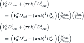
QED
14.3.9 Propulsive Efficiency
The power generated by an engine is not completely converted to a thrust force. It is inevitable that some losses occur in the process due to an imperfect conversion process. Consider an aircraft flying at an airspeed V generating thrust T by giving air a backward velocity w. This changes the kinetic energy of the affected air by an amount ½mw2 per unit time16 and this change must equal the force acting on the mass of air, times its speed, T·w. The term T·w is the power consumed (or wasted) in driving the air backwards. The Froude efficiency is defined as the ratio of the power required to propel an object (useful power) to the sum of this power and that which is lost in the conversion:
The Froude efficiency represents inviscid losses that result from accelerating the propwash. It is also called the ideal efficiency (see Section 14.5.2, Ideal efficiency). However, there are also losses due to the viscous drag of the propeller blades. These losses further increase the inefficiency of the power-to-thrust conversion process. This effect is called viscous profile efficiency and is denoted by the term ηv. We now define the total propeller efficiency, ηp, as the product of the Froude and profile efficiency as follows:
Propeller efficiency:17
![]() (14-34)
(14-34)
A typical maximum value for ηv is about 0.8 to 0.9.
The propeller efficiency can also be defined as the fraction of engine power that gets converted into propulsive power (thrust × airspeed) to the total engine output power, P. A common expression of this ratio is:
Derivation of Equation (14-35)
Using the definitions of the power and thrust coefficients, we write:
![]()
Inserting into Equation (14-22) and manipulating leads to Equation (14-23).
![]()
QED
Propeller Efficiency Map
Sometimes the propeller manufacturer will present the propeller efficiency in a mapped format similar to what is shown in Figure 14-34. In this format, the isobars represent constant values of propeller efficiency. Such maps are defined in terms of a specific propeller blade activity factor and are read as follows. First, determine the advance ratio using Equation (14-23). Then, determine the power coefficient using Equation (14-26). Finally, locate the value of the propeller efficiency using the two previous values. The propeller developer prepares such maps for different prop designs. The designer can review such maps for a specific propeller and decide whether it fits the desired performance of the aircraft.
It is evident that the propeller efficiency map does not lend itself to modern analysis methods. It is presented here merely for the sake of completeness. It is imperative that the data it represents be converted into a digitized format that allows the efficiency to be extracted using rapid computational approaches, using the modern spreadsheet or other numerical methods.
14.3.10 Moment of Inertia of the Propeller
As has been showed before, the moment of inertia of the propeller is of interest to the aircraft designer. This can be estimated using the fundamental definition for the moment of inertia of a body about a given axis:
![]() (14-36)
(14-36)
The term ρ·dV is the mass of an infinitesimal volume of the propeller blade, located a distance r from the reference axis (i.e. the axis of rotation of the propeller). While the planform of the propeller blade does not always yield an elegant closed-form solution of Equation (14-36), a reasonably accurate estimate of its moment of inertia can be made by idealizing each blade as a thin rod of a uniform cross-sectional area A (see Figure 14-35). If the radius of the prop is R, it weight is Wprop, and the number of blades is NB, then its moment of inertia can be estimated from:
![]() (14-37)
(14-37)
where g is the acceleration due to gravity.
Derivation of Equation (14-37)
The mass, m, of the propeller must be close to:
![]() (i)
(i)
where ρprop is the density of the material used in the propeller blades. Its mass can also be computed if its weight, Wprop, is known, i.e. from m = Wprop/g. It follows that the constant cross-sectional area is given by:
![]() (ii)
(ii)
Then, using Equation (14-36) we can compute the moment of inertia of a single rod extending from 0 to R:
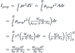
This result is for a single blade. If we have NB blades, this simplifies to:
![]()
QED
EXAMPLE 14-7
To evaluate this result of Equation (14-37), let’s compare it to the result using the standard expression for the moment of inertia of a thin rod. To do this determine the moment of inertia of a thin rod of mass m = 10 kg and length 2R = 2 m using each method.
Solution
Using the standard expression of moment of inertia we find that:
![]()
To prepare the method above, we note that the weight of the example rod is 10 × 9.807 = 98.07 N and its radius is 1 m. Therefore, using Equation (14-37) we get:
![]()
This is precisely what we would expect.
14.4 Determination of Propeller Thrust
The conversion of engine power to a propeller thrust force is not nearly as straightforward as that of the jet engine. This is due to the complex interaction between the propeller’s rotation speed, forward speed, and geometry. The designer can resort to a number of methods in order to estimate thrust, ranging from the simple to the complex. This section will present useful methods for this task.
14.4.1 Converting Piston BHP to Thrust
The performance analysis of piston engine aircraft requires brake horsepower (BHP) to be converted into thrust.18 In the UK system, the thrust is calculated using airspeed (in ft/s), engine power (in BHP), PBHP, and propeller efficiency (dimensionless), by solving Equation (14-23) for the thrust as follows:
![]() (14-38)
(14-38)
The factor 550 converts the BHP into ft lbf/s. In the SI system the conversion is not necessary as power is given in kW. The expression indicates that as the airspeed V approaches zero the thrust will trend toward infinity. This is physically impossible. What happens in reality can be understood by noting that the magnitude of the velocity through the propeller disc requires a constant flow of air toward it. This, in turn, means V is never zero. Thrust at zero forward airspeed can be estimated using the momentum theory (Section 14.5) or blade element theory (Section 14.6).
14.4.2 Propeller Thrust at Low Airspeeds
This section presents two methods to estimate propeller thrust at low airspeeds, which is essential for the prediction of low-speed operation such as that of T-O performance. Equation (14-38) is extremely useful in the performance analysis of aircraft. However, it presents an important difficulty to the user: it requires the propeller efficiency, ηp, to be known, but, being a function of the airplane’s airspeed, propeller geometry, and RPM, it is a hard number to estimate. Therefore, a more accurate way to write Equation (14-38) is shown below:
![]() (14-39)
(14-39)
where H is the altitude, Dp is the propeller diameter, RPM is the engine speed in revolutions per minute, MAP is the manifold pressure, and OAT is the outside air temperature. Naturally, this is far more cumbersome to write, which explains the short form shown in Equation (14-38).
The notion that ηp can be treated as a constant leads to a serious error in thrust calculations at low airspeeds because V is the denominator and it is becoming smaller, so the thrust grows unrealistically large. In performance analyses, low-speed performance cannot be ignored – for instance, it is needed to accurately predict take-off performance.
Method 1: Quadratic Interpolation
The quadratic interpolation method is based on the assumption that the propeller thrust varies from the static thrust at zero airspeed to the thrust at the maximum level airspeed (Vmax or VH) (whatever it comes out to be). This makes it possible to approximate the thrust using a quadratic polynomial of the form T = AV2+BV+C.
The method requires the propeller efficiency, ηp, at Vmax to be used. Figure 14-36 shows how the logic works, as applied to the SR22 (although this method should be limited to fixed-pitch propellers only). Equation (14-38) becomes hugely erroneous at low airspeeds and has a mathematical limit approaching infinity at V = 0 (a physical impossibility). The reader must keep in mind that the ηp in the figure is kept constant over the entire speed range, but this is only justifiable for the upper range of airspeeds, thanks to the airplane’s constant-speed propeller. In reality, the thrust ranges from TSTATIC at rest to Tmax at Vmax – a trend much better approximated by the quadratic interpolation formula, shown below:
![]() (14-40)
(14-40)
Derivation of Equation (14-40)
The goal of this derivation is to present a polynomial with three unknown variables, A, B, and C. This requires three independent equations:
At the first airspeed (V = 0):
![]() (i)
(i)
At the second airspeed (V = Vmax):
![]() (ii)
(ii)
where Tmax refers to the thrust at Vmax and not the maximum thrust possible (the static thrust). The slope at Vmax can be used to get the third equation, where the slope is calculated from:
![]()
Therefore, the third equation is:
![]() (iii)
(iii)
Equation (iii) gives:
![]()
Inserting this into Equation (ii) yields:
![]()
Algebraic manipulations yield:
![]()
Thus, the coefficient B can be rewritten as follows:
![]()
which allows us to combine the coefficients as follows:
![]()
QED
Method 2: Cubic Spline Method for Fixed-Pitch Propellers
Consider a performance analysis for an aircraft like the Piper J-3 Cub. The J-3 is powered by a 65 BHP Continental A-65 engine, has a stalling speed (VS) of about 33 KCAS, a cruising speed (VC) of about 65 KTAS, and a maximum speed (VH) of some 76 KTAS. A properly matched propeller should yield a ηp of 0.75 at around 65 KTAS, when the power is about 65% (42 BHP). On the other hand, it may be around 0.70 at the maximum airspeed of 76 KTAS. A typical J-3 propeller diameter is some 70 inches and, using Equation (14-63), the static thrust can be found to equal 546 lbf (not including the reduction factor 0.85 discussed in Section 14.5.3, Maximum static thrust). These values have been identified on the graph shown in Figure 14-37.
Figure 14-37 also shows thrust isobars for constant propeller efficiencies, ηp, at maximum power of 65 BHP. Note that the cruise point is slightly below the ηp = 0.5 isobar and not at 0.75 (as one might think at first, based on the previous paragraph). This is no mistake – the cruise power is based on 42 BHP and not 65 BHP. The isobars shown are based on full power. If they were based on 42 BHP they would all be sitting much lower and the cruise point would indeed be between 0.7 and 0.8 isobars. The two points to which the isobars pertain are labeled “Static Thrust” and “Max Airspeed.” The former is planted on V = 0 KTAS and T = 546 lbf and the latter on V = VH = 76 KTAS and the isobar where ηp = 0.70 (based on the assumption in the previous paragraph). It should be clear that as the airplane accelerates from standstill to maximum airspeed its thrust does not follow a particular isobar, but rather travels across them, showing that the propeller efficiency (and thrust) does indeed change with airspeed. Since propeller theory shows that the thrust is always less than the static thrust (see Section 14.4), whatever path the thrust follows between the two extremes, intuition holds that, generally, the change in thrust would move along a path indicated by the arrow shown in Figure 14-38. The question is only – how? Is this path a straight line or is it curved? Let’s try to answer those questions in detail.
Ultimately, the purpose here is to develop a tool that can be used to estimate the thrust for a fixed-pitch and constant speed propeller at a constant power setting with reasonable accuracy. This tool can then be used to estimate thrust at airspeeds as low as 0 ft/s, sorely needed for T-O analysis. The propeller thrust drops relatively sharply at first, but the drop is reduced as the airspeed increases. In other words, the derivative dT/dV is negative and steep at first; however, eventually it will level off as the airspeed and propeller efficiency increase. Since the maximum airspeed is usually an off-design point, dT/dV will become increasingly negative again. Based on the limited information we have (effectively static thrust and thrust or drag force at cruise and maximum airspeed) it is possible to represent this behavior using a cubic spline. This is the crux of the cubic spline method; it allows thrust to be approximated at a given power setting as a function of airspeed, using a cubic spline. A properly developed method allows such off-design conditions to be taken into account.
Such a cubic spline will be of the form:
![]() (14-41)
(14-41)
where the constants A, B, C, and D are determined using the following matrix equation:
 (14-42)
where the airspeeds VC and VH are in KTAS. The constants A, B, C, and D can be obtained by inverting the left square matrix and multiplying it by the array on the right-hand side. The use of this method will be demonstrated in Example 14-10 by applying it to the Piper J-3 Cub.
Derivation of Equation (14-42)
The trick is to determine the constants A, B, C, and D. To do this we need four equations. Observation shows that when V = 0, thrust is static thrust, TSTATIC. Using Equation (14-63), repeated here for convenience, we can easily write the constant D as follows:
![]() (14-63)
(14-63)
Note that it may be more appropriate to use Equation (14-64) rather than (14-63), as it better accounts for the effect of blockage, hub and tip, and the presence of the spinner. However, for this derivation the theoretical maximum static thrust is used. Since A2 = π·Dp2/4 and P = 550·PBHP, the first equation of the four can be written as follows (after a simple manipulation):
![]() (14-43)
(14-43)
Note that the power is the maximum power at the altitude. The next two equations are based on the airspeed for which the propeller has been optimized – here the cruising speed. Note, for a climb propeller it would be a different airspeed, although this should be denoted by VC as well. The importance of this airspeed is that this is where the propeller efficiency becomes a maximum. The assumption allows an additional equation to be generated, allowing the problem to be solved. The second equation of the four can now be written as follows:
Note that this equation uses the maximum power and not the cruise power, as this is the maximum thrust the engine would be capable of at VC. If the intent is to use airspeed in terms of KTAS rather than ft/s, Equation (14-44) must be rewritten as follows (note that in this case all the other equations must be in terms of KTAS as well):
The third equation is based on the fact that the propeller efficiency at VC, given by ηp max, is the highest it will become. This is where in ηp-V space the derivative dηp/dV = 0. In the T-V space the slope must be dT/dV at VC. This derivative can be calculated as shown below:
![]()
But by definition, at V = VC the derivative dηp/dV = 0; therefore:
Note that the units for the above derivative is in terms of lbf/(ft/s). If used with graphs such as that of Figure 14-37 or Figure 14-38, which are presented in terms of lbf versus KTAS, the derivative must be divided by 1.688 to convert the units to lbf/KTAS. This can be seen by noting that the derivative, when represented along the compressed KTAS axis, will be steeper by the factor 1.688. Therefore, to use Equation (14-46) with VC in terms of KTAS, use the following form:
This form is used with Equation (14-42) above. Thus, the third equation is based on the derivative at VC and is written as follows (here in terms of KTAS):
![]() (14-48)
(14-48)
Then, let’s consider the fourth and final equation, which describes thrust, TH, at maximum airspeed, VH. This expression requires the thrust to be determined by some means. Four ways come immediately to mind. (1) Use ηp provided by the propeller manufacturer to calculate thrust using Equation (14-38). (2) Estimate ηp using a method like the blade element theory (see Section 14.6) to calculate thrust. (3) Estimate ηp using (very good) engineering judgment based on knowledge of other airplanes to calculate thrust. (4) Calculate the drag of the airplane at the condition and use it as the thrust. Note that for a fixed-pitch propeller, ηp is less than ηp max. Assuming that ηp is known, we may write the fourth equation as follows:
These four equations can now be assembled into the following matrix form of Equation (14-42).
QED
EXAMPLE 14-10
Use the cubic spline method to determine a function T(VKTAS) that describes the full power thrust of the J-3 as a function of airspeed in KTAS. The maximum airspeed, VH, is 76 KTAS, where the thrust is 195 lbf, and static thrust, TSTATIC is 546 lbf. The propeller efficiency at cruise speed (VC) of 65 KTAS is assumed 0.75 and 0.70 at VH. Plot the resulting equation. Also plot the propeller efficiency that results from using the cubic spline.
Solution
Start by setting up the matrix of Equation (14-42):
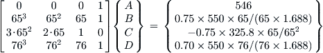
Evaluating the numbers yields:
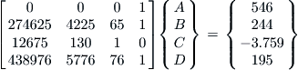
Inverting the matrix to solve for A, B, C, and D results in:

Therefore, the thrust at full power can be expressed as the following function of airspeed:
![]()
This is plotted in Figure 14-39. Note that the drag force for the J-3 has also been plotted, but it assumes the drag coefficient can be expressed using the simplified drag model, CD = CDmin + kCL2, where CDmin = 0.4976 and k = 0.05441, obtained from an unrelated analysis.
It can be seen the drag curve goes through both the 65% power cruise and maximum airspeed points, as is to be expected. The thrust curve T(V) intersects the max airspeed point only, which is in accordance with performance theory for steady level flight. Note how the cubic spline extends between the isobars of constant ηp = 0.7 and 0.8, indicating it captures the higher prop efficiency associated with VC.
To plot the propeller efficiency that results from using the cubic spline we simply back out the propeller efficiency based on Equation (14-38), that is:
![]()
The factor 1.688 is used to convert V, which so far has been in KTAS, to ft/s.This is plotted in Figure 14-40, showing the standard shape for propeller efficiency as a function of airspeed.
Method 3: Cubic Spline Method for Constant-Speed Propellers
The preceding treatment of the fixed-pitch propeller raises the question whether it can be extended to include constant-speed propellers. The answer is indeed yes. In particular, consider the unlikely design of a constant-speed propeller for the J-3 Cub. Say it is designed to generate a ηp of 0.85 at VC. It should be realized that one of the consequences of such a propeller is an increased cruising and maximum speed. Determining these two becomes one of the primary tasks in applying the method to constant-speed propellers.
For the most part, this method is identical to the one for the fixed-pitch propeller. It also uses Equation (14-42) with one major difference; the new VC and VH must be determined. This can be done if we assume that the ηp at VH will be the same as that at VC. The justification can be seen in Figure 14-48. It shows that the nature of constant-speed propellers is to yield a relatively constant ηp at high airspeeds. The determination of VH requires the drag properties of the aircraft to be known. If so, the method of Section 19.2.14, COMPUTER CODE: Determining maximum level airspeed, Vmax, for a propeller aircraft, can be used to estimate both VC and VH. Then, Equation (14-42) can be populated and the constants A, B, C, and D of the cubic spline of Equation (14-41) determined. The use of this method will now be demonstrated by, again, applying it to the Piper J-3 Cub.
EXAMPLE 14-11
Use the cubic spline method to derive a function, T(VKTAS), that describes the thrust of the J-3 at full power using a constant-speed propeller designed to give a propeller efficiency of 0.85 at cruise and maximum airspeed. Also plot the propeller efficiency that results from using the cubic spline.
Solution
By using the computer code of Section 19.2.14 the cruising speed at 65% power and maximum airspeed of the J-3 with the new propeller was estimated to equal 68.7 and 81.6 KTAS, respectively. The corresponding thrust (using ηp = 0.85) were found to equal 262 and 221 lbf, respectively. The same static thrust, TSTATIC = 546 lbf, is used. Note that since the method was implemented using Microsoft Excel it is not possible to display all the decimals retained by the program. Then, set up the matrix of Equation (14-42):

Evaluating the numbers yields:
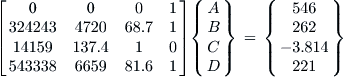
Inverting the matrix to solve for A, B, C, and D results in:
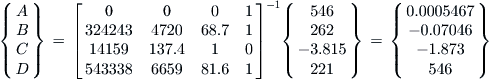
Therefore, the thrust at full power can be expressed as follows:
![]()
This is plotted in Figure 14-41. The drag force and the thrust curve for the fixed-pitch propeller have also been plotted to better realize the difference between the two thrust curves. Again, this assumes the drag coefficient can be expressed using the simplified drag model, CD = CDmin + kCL2, where CDmin = 0.4976 and k = 0.05441, obtained from an unrelated analysis.
To plot the propeller efficiency that results from using the cubic spline, the same method is used, as was shown in Example 14-11; we simply back out the propeller efficiency based on Equation (14-38), that is:
![]()
This is plotted in Figure 14-42, showing the standard shape for propeller efficiency for a constant-speed propeller as a function of airspeed. It can be seen the general shape is maintained up to VH, as the spline is forced into the appropriate shape, after which an error begins to creep in; therefore, do not extrapolate the thrust.
It is important to understand that while the new propeller efficiency deviates at airspeeds higher than VH, the method still provides a simple means to perform performance analysis with acceptable accuracy at other airspeeds. It is possible to improve the shape of the spline by fitting a quartic or higher-order spline through the known data, although this becomes progressively more cumbersome. It appears that a cubic spline offers the right amount of complexity and practicality for this kind of analysis.
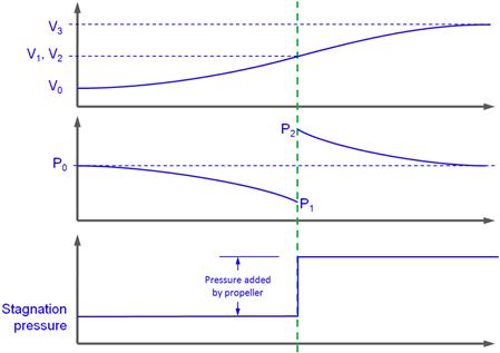
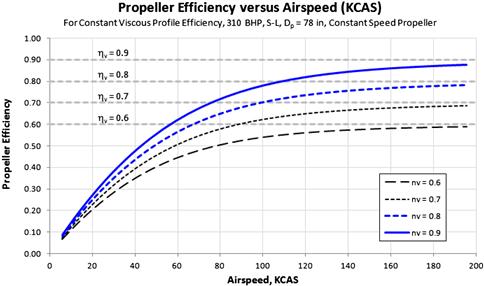
14.4.3 Step-by-step: Determining Thrust Using a Propeller Efficiency Table
Sometimes the propeller manufacturer provides the designer with a propeller efficiency table like the one shown in Figure 14-43. In it the propeller efficiency can be read based on the computed value of the advance ratio (left-most column) and power coefficient (top row). Using such a table presents a very convenient way to extract the propeller efficiency for use with Equation (14-38). To do this the user must calculate the power coefficient, CP (defined in Section 14.3.7, Definition of power- and thrust-related coefficients), and advance ratio, J (defined in Section 14.3.5, Advance ratio), and use these to extract the prop efficiency. The sample table below has the advance ratio in rows, ranging from 0.20 to 1.20, and the CP in columns, ranging from 0.02 to 0.13. Values of J or CP that fall between the tabulated values must be extracted by double-interpolation.
Using such a table, the method of extracting thrust is as follows:
Step 3: Extract Propeller Efficiency
Use a method such as the one in Section E.5.11, Step-by-step: Rapid interpolation of 2D lookup tables, to extract the propeller efficiency, using the calculated CP and J.
Step 4: Calculate Thrust
Calculate thrust from Equation (14-38):
![]()
EXAMPLE 14-12
An airplane is equipped with a 70′′ diameter constant-speed propeller driven by a 150 BHP piston engine. If flying at sea-level at 130 KTAS with the prop swinging at 2700 RPM and max power, using the table in Figure 14-43, what is the magnitude of the thrust?
14.4.4 Estimating Thrust From Manufacturer’s Data
As said earlier, it is always wise for the aircraft designer to establish a good relationship with propeller manufacturers by committing to using their products. Such relationships may (1) encourage the propeller manufacturer to provide the designer with useful propeller performance information, and (2) if the business case is promising enough, even persuade the manufacturer to design a propeller to match the designer’s desired characteristics.
An example of typical data provided by a propeller manufacturer is shown in Figure 14-44. The data is for a two-bladed, 69 inch diameter propeller designed for an LSA aircraft. These propeller characteristics are plotted in Figure 14-45, with the appropriate curve fits. So, now we have the properties of the propeller formulation as a function of advance ratio.
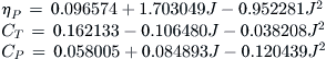
EXAMPLE 14-13
An airplane is equipped with a 69′′ diameter fixed-pitch propeller driven by a 100 BHP piston engine. If flying at sea-level at 110 KCAS with the prop swinging at 2400 RPM and 75% power, using the above equations, what is the magnitude of the thrust?
14.5 Rankine-Froude Momentum Theory
The momentum theory is a mathematical method that models the performance of a propeller. It is also known as the actuator disc theory. The theory was originally developed in 1865 by the famed Scottish physicist William John Macquorn Rankine (1820–1872), who had a particularly prolific career as a scientist and to whom the Rankine temperature scale is credited. Important contributions were made by the English hydrodynamicist William Froude (1810–1879). Rankine’s contribution is generally dated to 1865, and that of Froude over the period from 1878 to 1889 [9].
The theory can be used to estimate propeller thrust, although the results are generally optimistic. It allows the airspeed inside the propeller streamtube to be estimated (the so-called propeller-induced velocity), which is an important result used with the blade element theory, introduced in Section 14.6. The momentum theory is based on the following assumptions:
(1) The propeller is replaced by an infinitesimally thin actuator disc that offers no resistance to air passing through it.
(2) The disc is uniformly loaded and, therefore, experiences uniform flow passing through the actuator disc. Consequently, it is assumed to impart uniform acceleration to the air passing through it.
(3) A control volume surrounds the streamtube and sharply separates the flow going through it from the surrounding air.
(4) Flow outside the streamtube has constant stagnation pressure (which means no work is imparted on it).
(5) In the far-field, in front and behind the disc, streamlines are parallel and, there, the pressure inside the streamtube is equal to the far-field pressure.
(6) The propeller does not impart rotation to the flow.
(7) The theory assumes inviscid (no drag, no momentum diffusion) and incompressible flow.
14.5.1 Formulation
Consider Figure 14-46, which shows an idealized flow model for the actuator disc. The model consists of the four planes; ![]() ,
, ![]() ,
, ![]() , and
, and ![]() . From Assumption (5), Plane
. From Assumption (5), Plane ![]() is far enough ahead of the actuator disc for the streamlines to be parallel. Plane
is far enough ahead of the actuator disc for the streamlines to be parallel. Plane ![]() is far enough behind the disc for the streamlines to have become parallel again. Consequently, the static pressure at either plane is constant and equal to the far-field pressure P0.
is far enough behind the disc for the streamlines to have become parallel again. Consequently, the static pressure at either plane is constant and equal to the far-field pressure P0.
The front face of the control volume has surface area S. The flux of fluid entering through Plane ![]() is Q0 = S·V0. The flux exiting through Plane
is Q0 = S·V0. The flux exiting through Plane ![]() is Q3 = (S − A3)·V0 + A3·V3. The change in flux between the front and aft surfaces is thus given by:
is Q3 = (S − A3)·V0 + A3·V3. The change in flux between the front and aft surfaces is thus given by:
![]()
The non-zero value of the flux implies fluid must be entering the control volume from the sides. Now in order to determine the thrust it is necessary to apply the momentum theorem, repeated here in its conventional form;
![]() (C-19)
(C-19)
where n = normal vector to the cross-sectional area
Note that the momentum flux of the fluid entering Plane ![]() is given by
is given by ![]() (the negative sign indicates it is entering the volume). Similarly, the momentum flux of the fluid entering Plane
(the negative sign indicates it is entering the volume). Similarly, the momentum flux of the fluid entering Plane ![]() is given by
is given by ![]() (the positive sign indicates it is leaving the volume). Finally, the momentum flux of the fluid entering the sides is given by
(the positive sign indicates it is leaving the volume). Finally, the momentum flux of the fluid entering the sides is given by ![]() (the negative sign indicates it is entering the volume). This generates a force that points in the direction of the incoming flow (here renaming F as T for thrust):
(the negative sign indicates it is entering the volume). This generates a force that points in the direction of the incoming flow (here renaming F as T for thrust):
![]()
Inserting our previous result for ΔQ leads to:
![]() (14-51)
(14-51)
Considering Figure 14-46 it can be seen that T can also be computed from:
![]() (14-52)
(14-52)
where
The changes in pressure and airspeed are depicted in Figure 14-47. It can be seen that the propeller energy is added as a rise in stagnation pressure. Its magnitude depends on the geometry of the propeller and the power delivered by the power plant.
We can calculate P1 and P2 using Bernoulli’s principle assuming streamlines exist up to the actuator disc and immediately behind it. We must note this principle is not applicable through the actuator itself, although it is reasonable to assume the velocity is continuous through the disc. Thus, we can determine P1 using the flow conditions at Plane ![]() , and P2 using the flow conditions at Plane
, and P2 using the flow conditions at Plane ![]() as follows:
as follows:
From which we find the pressure difference by subtracting Equation (i) from (ii).
![]()
Note that since V1 = V2 we can simplify:
![]() (14-53)
(14-53)
Now, insert Equation (14-53) into (14-51) to get:
![]() (iii)
(iii)
Equate this with Equation (14-51):
![]() (iv)
(iv)
![]() (v)
(v)
![]() (vi)
(vi)
![]()
![]() (vii)
(vii)
![]() (14-54)
(14-54)
The above equation is recognized as Froude’s Theorem [10] and is essential in propeller design. It states that the airspeed through the propeller is the average of the far-field airspeed (V0) far ahead of it and the airspeed in the streamtube far behind (V3). Let’s now define the following differences:
![]() (viii)
(viii)
where w is called the propeller-induced velocity. This allows V2 to be redefined as follows:
![]() (ix)
(ix)
and V3 as:
![]() (x)
(x)
Inserting Equations (ix) and (x) into Equation (14-51) results in:
![]()
The power for this system is given by P = T·V or;
![]() (14-56)
(14-56)
The above result shows the power required by the propeller is a combination of two terms; useful power and induced power:
We can determine the induced velocity, w, through the propeller disc from Equation (14-55):
![]()
This is a quadratic equation in terms of w and can be solved using Equation (E-12):
![]()
Simplifying and recognizing the negative sign in front of the radical represents a non-physical condition, we write this as:
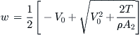 (14-57)
Using the above analysis, we can consider two important cases; ideal efficiency and maximum static thrust.
14.5.2 Ideal Efficiency
Ideal efficiency can be defined as the ratio of useful power (Equation (xi)) to the total power per Equation (14-56):
![]() (14-58)
(14-58)
We can introduce the fraction w/V0 to Equation (14-57), yielding:
![]() (xv)
(xv)
where CT is the coefficient of thrust (not to be confused with the thrust coefficient of Equation (14-27)) as follows:
![]() (14-59)
(14-59)
Inserting this into Equation (xiv) leads to:
![]() (14-60)
(14-60)
14.5.3 Maximum Static Thrust
Consider the special case when V0 = 0. In this case, Equation (14-57) the velocity through the propeller reduces to:
![]() (14-61)
(14-61)
Similarly, the power from Equation (14-56) becomes:
![]() (14-62)
(14-62)
This yields the following expression for static thrust, TSTATIC:
![]() (14-63)
(14-63)
As a rule of thumb, Equation (14-63) overestimates static thrust by some 15–20% for various reasons, such as blockage effects, the presence of the hub, which reduces the disk area, reduction of lift distribution near the tip and hub, and so on. Therefore, for design purposes, for typical aircraft, estimate TSTATIC by the following empirical correction:
![]() (14-64)
(14-64)
EXAMPLE 14-14
A two-bladed propeller whose diameter is 76′′ is observed to generate 1500 lbf of thrust. What is the pressure rise (ΔP) through the propeller disc according to the momentum theory?
EXAMPLE 14-15
An airplane is powered by a two-bladed propeller whose diameter is 76′′ is driven by a 310 BHP engine. What is the maximum static thrust one can expect from it at sea-level? What is the static thrust if the spinner diameter is 18′′? What is the speed of air through the propeller disc?
Solution
Using Equation (14-63) we determine the maximum static thrust as follows:
![]()
Static thrust corrected for spinner:
![]()
The speed of air through the propeller disc is found from Equation (14-61):
![]()
The static thrust in the example is overestimated as it does not account for the fact that the distribution of lift along the blade of the propeller is not constant and necessarily becomes zero at the tip. Thus the value represents a theoretical upper limit on the thrust.
EXAMPLE 14-16
The aircraft of the previous example is cruising at 185 KTAS at 8000 ft at a power setting of 233 BHP and it has been estimated its drag amounts to 470 lbf. What is the propeller efficiency?
Solution
Air density at 8000 ft from Equation (16-18):
![]()
Assuming T = D we get the following value for the coefficient of thrust:
![]()
Therefore, the prop efficiency is:
![]()
EXAMPLE 14-17
The propeller of Example 14-15 is found to generate 556 lbf of thrust at 160 KTAS (270.1 ft/s). Determine the induced velocity and ideal efficiency at that condition.
Solution
Area was determined to be 31.50 ft2 in Example 14-15. Therefore, the induced velocity is found from Equation (14-57):

The ideal propeller efficiency is found from Equation (14-60):
![]()
Just as in the case of the static thrust, the propeller efficiency is overestimated as well. The example above is for an airplane in the Cirrus SR22/Cessna Corvalis class, for which a more accurate efficiency is in the 0.86–0.88 range for the cited flight condition.
14.5.4 Computer code: Estimation of Propeller Efficiency Using the Momentum Theorem
Propeller efficiency is required to predict the performance of propeller-powered aircraft. During the development of such aircraft, the designer must be able to predict with a reasonable level of accuracy the propeller efficiency. One way of doing this is to use the blade element theory (BET), which is presented in Section 14.6, Blade element theory. However, there are times, in particular during the early phases of development, during which it may simply seem too unwieldy. This is due to the fact that detailed information about the geometry of the propeller must be known in advance, but this may be impossible at that stage of development when perhaps the only thing known is that the airplane will be powered by a propeller. The following method, which uses the momentum theorem, is intended to remedy this problem. As such, it is far simpler to implement than the BET, although it is also best implemented using software such as a spreadsheet or mathematical script software like MATLAB. Here, a function written in Visual Basic for Applications (VBA), intended for use with Microsoft Excel, is presented.
The momentum theory can also be used to extract propeller efficiency from flight test data. To do this, details of the flight condition (airspeed, altitude, etc.) and power setting are recorded and reduced in the manner shown below. It must be kept in mind that initially, neither thrust, T, nor propeller efficiency, ηp, is known. The method requires the viscous profile efficiency, ηv (see Section 14.3.9, Propulsive efficiency) for the propeller to be known. Its value may be provided by the propeller manufacturer and typically ranges from 0.7 to 0.9, depending on propeller type (i.e. fixed or constant speed) and geometry. Sometimes it is given as a function of airspeed. From a certain point of view it can be considered the maximum value or ceiling of the propeller efficiency, ηp.
We begin the process by estimating token thrust using some initial value of the propeller efficiency, denoted by ηp. This is then used to estimate the induced airspeed in the propeller streamtube, which, in turn, is used to calculate the ideal propeller efficiency. This is then used to calculate the new propeller efficiency, ηpnew, as the product of the ideal and the viscous profile efficiencies. If the difference between the original and new values is larger than some selected level of accuracy (e.g. 0.0001) then the value of ηp is replaced with that of ηpnew and the process is repeated until the difference has reached the desired accuracy.
Step 1: Preliminaries
Establish power, P, airspeed, V, altitude, H, propeller disc area, A, and the estimated viscous profile efficiency.
Step 2: Set Initial Values
Set an initial value for the propeller efficiency, ηp. For instance, start with ηp = 0.5. Also, estimate the propeller profile efficiency, ηv. In the absence of an analysis use ηv = 0.85.

Step 6: Determine the Next Propeller Efficiency
Recalculate new propeller efficiency:
![]()
Step 7: Determine the Change in Propeller Efficiency
Calculate the difference between the new and original propeller efficiencies:
![]()
Step 8: Plan the Next Step
If the difference, Δ, is larger than, say, 0.0001 then set ![]() and return to Step 3.
and return to Step 3.
If the difference, Δ, is less than 0.0001 then stop.
The following Visual Basic subroutine (or function) implements the above methodology and can be used without modification in Microsoft Excel. The function is written as a VBA (Visual Basic for Applications) function and can then be referenced from within Excel as any other function (e.g. SIN(), COS(), etc.). The arguments (BHP, V, H, etc.) can be cell references (e.g, E4, E5, etc.) or number.
Using this routine, it is possible to estimate the propeller efficiency as a function of airspeed. There are a few caveats though. For instance, the magnitude of the variable ηv (the viscous profile efficiency), denoted by Nv in the VBA function, functions as a limit on the magnitude of the ideal propeller efficiency, ηi, denoted by Ni. This is shown in Figure 14-48 and shows how the total propeller efficiency becomes an asymptote to the value of ηv, indicating this is the maximum value it can acquire. This would be possible only if the ideal efficiency could reach 1. The arguments (W, Dp, and BHP) of the curves in Figure 14-48 correspond to those of the SR22, which has been used throughout this book as an example aircraft.
A more realistic scenario is one in which ηv is not constant, but a function of the airspeed. Such effects can be attributed to viscosity at lower airspeeds and compressibility effects at higher airspeeds. Both affect the shape of the resulting propeller efficiency in profound ways, as can be seen in Figure 14-49. The graph shows how the airspeed changes modify the ηv and lead to a distinct maximum value of the propeller efficiency, rather than a horizontal asymptote. The effect can be extended to fixed-pitch propellers by the proper selection of a curve that describes the changes in the viscous profile efficiency. In this way the propeller efficiency can be forced into a shape that is a reasonable approximation of the real propeller, allowing for more precise performance estimation.

The reader must be mindful that this method is simply a tool intended to make the performance analyses of propeller aircraft easier in the absence of actual manufacturer’s data. Of course, in order for it to be practical, it must align well with real data. For instance, we might know that a given propeller is optimized at a given airspeed. Judging from whether the propeller is a fixed or constant-speed propeller, we might guess that its maximum prop efficiency is, say, 0.75 for a fixed pitch and 0.85 for a constant-speed prop. The curve representing ηv should then be selected such that at a low airspeed the product ηv·ηi is about 0.1 and at intended cruising speed (for which the propeller is optimized) the product reaches the maximum values (0.75 or 0.85). At a higher airspeed this would be reduced.
14.6 Blade Element Theory
The blade element theory (BET) attempts to estimate the thrust of a propeller by dividing each blade into a number of segments, called blade elements. The theory treats each element as an independent two-dimensional airfoil, which allows the aerodynamic forces to be calculated based on the local flow conditions at the element. Then, once the aerodynamic properties have been determined, they are summed up to evaluate the properties of the complete propeller. Propellers usually feature morphing airfoil shapes, as the airfoil changes gradually from a thick airfoil at the hub to at thin one at the tip. The blade element theory can handle any such changes, although solution schemes must be prepared with such changes in mind.
The BET was first devised by the Polish scientist Stefan Drzewiecki (1844–1938), who between 1892 and 1920 almost entirely developed the so-called primitive blade element theory, which was published in 1920 in his book Théorie Générale de L‘Hélice [11] (General Theory of Helixes). This simplified theory ignored the presence of the induced flow inside the propeller streamtube [12]. Consequently, predicted thrust is higher than experimental thrust at the same condition. The method was improved by a contribution from William Froude (1810–1879), himself one of the two people behind the momentum theory (see Section 14.5, Rankine-Froude momentum theory). An accurate depiction of the propeller is realized by the BET only through an estimation of the so-called propeller-induced velocity, which changes the AOA seen by the blade elements. This is caused by the fact that the airspeed inside the propeller streamtube moves faster than the surrounding air. One way of modeling this effect is to use the momentum theory to describe the induced velocity inside the streamtube.
The BET offers a number of advantages when compared to the momentum theory. It can account for varying blade geometry, change in the airfoil’s chord, angle-of-pitch, and aerodynamic characteristics. It allows torque to be estimated, which allows the designer to determine the power required to swing it. It also allows important non-linearities, such as that of a standard lift curve, to be modeled. These are the primary reasons for the method’s popularity in propeller design.
The BET also suffers from a number of limitations. The theory assumes the flow inside the streamtube is uniform, which does not hold for distorted streamtubes (for instance, blockage effects). The assumption that the forces on each blade element can be treated as two-dimensional neglects spanwise flow. Spanwise flow is important if large pressure gradients exist along the propeller blade. The theory assumes the flow is mostly steady and, therefore, does not model thrust lag caused by change in operating conditions (e.g. change in RPM). The theory also assumes the blade is rigid, ignoring aeroelastic effects. Also, it is a drawback that a special correction has to be made at the hub and tip to account for diminished lift and for a skewed inflow, such as a propeller at a high AOA (e.g. see Figure 14-17).
14.6.1 Formulation
Figure 14-50 shows a propeller of a radius R rotating with an angular velocity of Ω radians/sec. A representative blade element is shown whose chord is denoted by c(r) and width by dr. Its centerline is located at a distance r. A cross-sectional view of this blade element, detailing airspeed components and angles, is shown in Figure 14-51.


The following parameters are identified in Figure 14-51:
| r = | arbitrary distance from hub to blade element |
| V0 = | forward airspeed of the airplane |
| VE = | effective resultant velocity |
| VR = | resultant velocity |
| w = | elemental induced velocity; due to flow in the streamtube being faster than the far-field airspeed |
| Ω = | angular velocity of the propeller |
| α = | elemental angle-of-attack |
| αi = | induced angle-of-attack that results from the induced velocity of air |
| αZL = | airfoil’s zero lift angle |
| β = | pitch angle, which is defined as the angle between the rotation plane and the zero lift line of the blade element airfoil |
| ϕ = | helix angle |
The differential lift and drag forces of the element, dL and dD, can now be written as follows:
![]() (14-65)
(14-65)
![]() (14-66)
(14-66)
where
c(r) = chord at blade station r, in ft or m
Cd = section drag coefficient of the element airfoil
The section lift coefficient of the element airfoil can also be written as follows:
![]() (14-67)
(14-67)
where the helix angle is calculated from the relation:
![]() (14-68)
(14-68)
Observation 1
Note that the CL-α tables for airfoils for ordinary lifting surfaces always use the chordline as datum, whereas for propeller airfoils the zero-lift line is the datum. This must be accounted for when determining the lift and drag coefficients using such data.
Also note from Figure 14-51 that dL is perpendicular to the vector VE and dD is normal to it. With that in mind, the differential thrust, torque, and power can be calculated as follows. Recall the definition of power as force × speed. Therefore, the power applied to each blade element equals the amount required to move it through air with force dFQ at a speed Ω·r:
This allows us to calculate thrust and torque as follows:

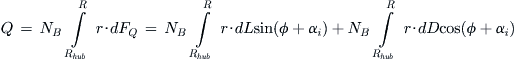
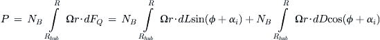
where NB is the number of propeller blades, R is the tip radius and Rhub is the hub radius. Note that in the UK system the unit for torque is ft·lbf and ft·lbf/s for power. In the SI system the units are N·m (or J) and N·m/s (or W), respectively.
The remaining problem is to determine the induced AOA and its effect on the thrust and torque. It can be seen in Figure 14-51 that the presence of w will reduce the AOA and thus modify the thrust and torque.
The reader should recognize that modern-day methodologies do not evaluate the integrals of Equations (14-72) through (14-74) directly, but rather solve them using numerical integration. This is easy to accomplish using the modern-day spreadsheet or a computer program. Spreadsheet methods increase flexibility and arguably result in improved accuracy, because a number of simplifications would have to be made in order to allow the resulting integrals to be evaluated (for instance when incorporating the helix angle). Additionally, an explicit integral solution would have to be prepared for any individual geometry, whereas a spreadsheet formulating the numerical integration method can be easily modified to incorporate any geometric complexity desired. This is the approach that will be used in this text. The following example displays how such a spreadsheet is constructed and incorporates real complexities such as a tapered blade chord, variable pitch angle, and drag coefficient which is a function of the lift coefficient.
EXAMPLE 14-18
Determine the thrust, torque, and power for a three-bladed propeller whose diameter is 76 inches, hub diameter is 12 inches, a chord whose linear taper is described by the expression 6−2r/R inches, and pitch which varies linearly from an angle of 65° at the hub to 20° at the tip. The propeller is rotating at 2500 RPM at a forward speed of 160 KTAS at S-L. The propeller’s airfoil is a Clark Y, whose lift and drag coefficients are given by NACA R-502. Initially, assume that the induced velocity, w, is 0, but account for the non-linearity of the lift and drag coefficients.
Note that this example assumes there is no propeller-induced velocity inside the streamtube. As such, it represents the results of Drzewiecki’s primitive blade element theory. The next example demonstrates the effect of introducing propeller-induced velocity on the derived properties.
Solution
The primary purpose of this problem is to show how to extract propeller properties using the blade element theory, and help the reader understand the importance of accounting for the induced flow field going through the propeller. For this reason it is also important the reader also studies Examples 14-19 and 14-20.
This problem will be solved numerically and is prepared as shown in the table in Figure 14-53. In the interests of space, the table will be broken into three sub-tables, consisting of columns 2–9, 11–17, and 18–25, and each will be given more space so their content is legible. Note that the blue shading in row 10 indicates the values that are calculated as detailed below. However, before we start we must calculate several preliminary values that must be used to complete the table.

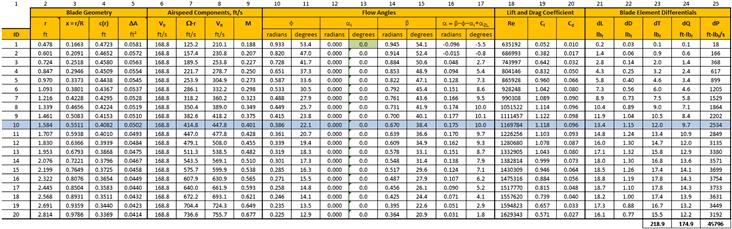
The solution as prepared here breaks the propeller blades into 20 elements of equal width. Let’s begin the procedure by calculating some preliminaries:
![]()
![]()
![]()
![]()
![]()
![]()
Thus, the first blade station in Figure 14-54 (see row 1), is the hub radius plus one half of the element width because the radials are positioned at the center of the elements (see Figure 14-52). Keeping in mind that numerical subscripts refer to the row number, we get:
![]()

Consequently, subsequent blade stations can be calculated by simply adding Δr to the previous blade station.
Step 1: Table Columns 2–9
Refer to Figure 14-54. Column 2 is calculated for each row by adding the element width Δr to the blade station (or radial) in the previous row. For example, to calculate the radial in row 10, we look at the value in row 9, which equals 1.633 and add Δr to it, or:
![]()
Column 3 is calculated to allow plotting of results with respect to the fraction of the blade span (see for instance Figure 14-58). The value in row 10 is calculated as follows:
![]()
Column 4 is the chord at the radial and for row 10 is calculated as follows:
![]()
Column 5 is the area of the blade element in row 10 and is calculated as follows:
![]()
Column 6 is the forward speed (i.e. the airplane’s airspeed) converted to ft/s, i.e. 160 KTAS × 1.688 = 270.1 ft/s and is equal for all the rows. Column 7 is the blade’s rotational speed and is calculated as follows for row 10:
![]()
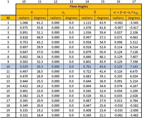
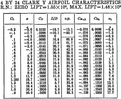
FIGURE 14-56 Original data from Ref. 13 used to model the propeller airfoil.
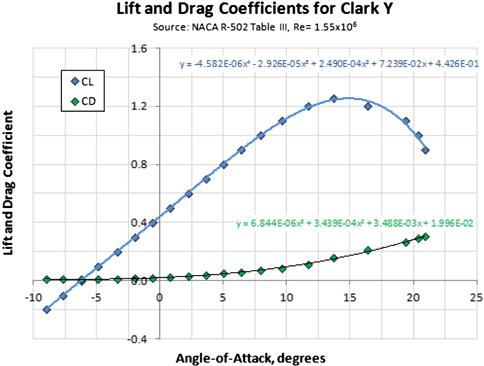
FIGURE 14-57 Original data from Ref. 13 plotted and curve-fitted.
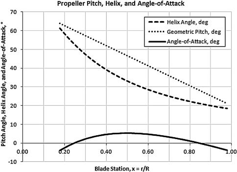
VR is given by Equation (14-9) and is calculated in column 8. The value in row 10 is found from:
![]()
Finally, the Mach number is calculated in column 9 and for row 10 is found to equal:
![]()
Step 2: Table Columns 11–17
The next sub-table contains the flow angles, as shown in Figure 14-55. Columns 10 and 11 contain the helix angle in radians and degrees, respectively. For rows 10 and 11 this is calculated as follows:
![]()
Columns 12 and 13 contain the induced flow angle, αi, ahead of the propeller, which reduces the overall AOA on the blade element. As stated in the introduction to the problem, it is assumed that the induced velocity equals zero. We will study in Example 14-19 the impact of a non-zero induced velocity on the thrust, torque, and power. At any rate, since w = 0 the values in columns 12 and 13 are all zero.
Columns 14 and 15 contain the geometric pitch angle β which is specified as 65° at the hub (r = 0.5 ft) and 20° at the tip. Using the parametric formulation of Appendix E.5.5 we write:
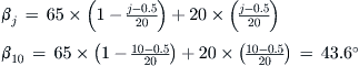
Note that 0.5 is subtracted from the row index because when j = 1 (row 1) the parameter should be zero, but we are at the middle of the first element. Columns 16 and 17 contain the AOA of the airfoil. Referring to Figure 14-55 we see that α is determined from Equation (14-36) as follows:
![]()
However, as mentioned in OBSERVATION 1 in the derivation section, the aerodynamic data obtained from NACA R-502 [13], which is used to calculate the section Cl and Cd, uses the chordline for reference datum (see Figure 14-56) rather than the zero-lift AOA line. For this reason the expression must incorporate a correction as shown below:
![]()
Where αZL is the zero lift AOA and amounts to −6.2° as can be seen in Figure 14-56 or Figure 14-57. Therefore, for row 10 we get the following AOA:
![]()
The resulting angles are shown plotted versus the blade station in Figure 14-58.
Step 3: Table Columns 18–25
Column 18 contains the Reynolds number for the blade elements and is calculated from Equation (8-29) (which is only valid for S-L, where the analysis is performed):
![]()
The Re for the propeller ranges from approximately 930,000 to 1,840,000. For this reason Table III of NACA R-502 was selected (Figure 14-56) as it contains airfoil properties at Re between these extremes. The Cl and Cd in Table III are plotted in Figure 14-57 and curve-fitted using a best-fit polynomial. These curve-fits are presented below and calculated for row 10 using the previously calculated α = 7.1° for that station:
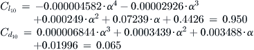
Columns 21 and 22 contain the differential lift and drag acting on the element and are calculated using Equations (14-65) and (14-66). For row 10 this becomes:
![]()
![]()
Column 23 contains the differential thrust calculated using Equation (14-69):
![]()
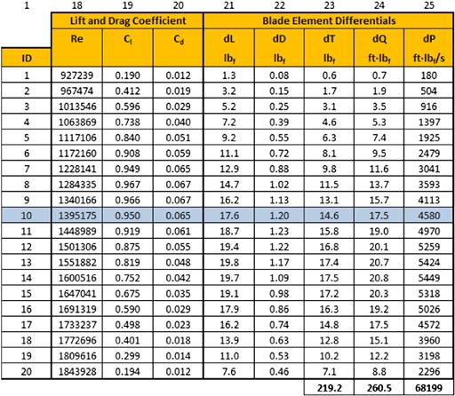
Column 24 contains the differential torque calculated using Equation (14-70):
![]()
Column 25 contains the differential thrust calculated using Equation (14-71):
![]()
Once all the rows have been calculated in this fashion the next step is to sum up the dT, dQ, and dP, but the sum is the thrust, torque, and power generated by a single blade. These values must be multiplied by 3 to account for the three blades on the propeller. The resulting values are:
We can calculate additional information as shown below:
Finally, note that the power can also be calculated using the torque coefficient as follows:
![]()
![]()
EXAMPLE 14-19
Using the spreadsheet of Example 14-18 determine, tabulate, and plot the variation of T, Q, P, ηp for non-zero values of induced velocity, such that αi ranges from 0.5° to 5° stepping through a 0.5° interval. The purpose of this example is to evaluate the influence of the induced airspeed on the above parameters. Note that these angles are entered for demonstration only. Example 14-20 estimates these angles using the momentum theory.
Solution
The results are tabulated below and plotted in Figure 14-60. We can see that the induced velocity significantly affects all of the parameters requested.
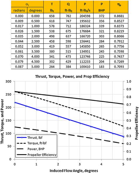
The aircraft designer should be aware of and concerned with such changes. Even a modest change in the induced flow angle, from 0° to 2°, reduces thrust from 219 lbf to 166 lbf, by almost 25%! Additionally, the blade element method does not include tip effects, which may reduce thrust by additional 10% or so. This shows that ignoring this flow-field phenomenon has a major effect on accuracy and must be taken into account. This effect will be formulated in Section 14.6.4, Step-by-step: Prandtl’s tip and hub loss corrections.
14.6.2 Determination of αi Using the Momentum Theory
Having demonstrated the importance of induced AOA, αi, on propeller thrust and power (see Example 14-18), we will now develop a method to help determine the induced velocity, w. One way of accomplishing this is to use the actuator disc or momentum theory (see Section 14.5). Considering Figure 14-51 we see that αi depends on w, which, in turn, depends on the blade loading. The method shown here is best implemented in a spreadsheet or a computer program. We will incorporate it into the spreadsheet just developed in the preceding examples.
Consider the propeller of Figure 14-61. A circular area (or annulus) of width dr located at blade station r is shown. The total area of the annulus is dA = 2πr·dr. The total thrust of the propeller using the Rankine-Froude momentum theory of Section 14.5 is given by Equation (14-29), repeated here for convenience:
![]() (14-75)
(14-75)
where

Therefore, the thrust generated by the annulus according to the momentum theory is:
![]() (i)
(i)
However, dT is also defined by the blade element theory using Equation (14-38). Using that expression and by combining Equations (14-34) for dL and (14-35) for dD and noting that dT is the product of the number of blades, NB, we get:
![]()
Considering Figure 14-51 again shows that we can make the following approximations for VE, w, and the angle ϕ+αi:
![]() (iii)
(iii)
![]() (iv)
(iv)
![]() (v)
(v)
![]() (vi)
(vi)
Insert this into Equation (ii) to get:
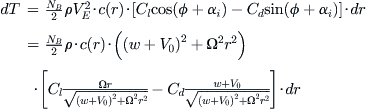
It must be pointed out that the induced flow angle will reduce the value of the Cl and consequently change the magnitude of Cd. This, in turn, will change the loading on the blades and therefore affect the induced velocity.
Equating Equations (i) and (vii) leads to (rewrite c(r) = c for clarity):
![]()
Canceling terms and expanding:
![]()
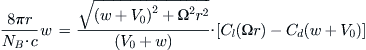
The purpose of these manipulations is to ultimately retrieve the value of w at a given radial station r. Equation (viii) is best solved by an iterative scheme, such as Newton-Raphson (see Appendix E.6.19), but this also requires a specific function, call it f(w), and its derivative, i.e. f′(w).
Let’s define a function f(w) as follows:
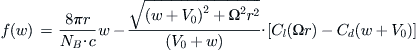 (ix)
(ix)
Rewriting it using the definition of VE we get:
![]() (14-76)
(14-76)
The derivative of f(w) is determined as follows:
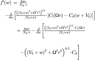
Carrying the differentiation further:
 (x)
(x)
Differentiate the right-most term using the chain rule (see Appendix E.6.2),
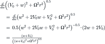
Differentiate the center term:
![]()
Completing differentiating the center term leads to:
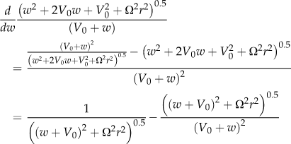
Insert into Equation (x) and manipulate.
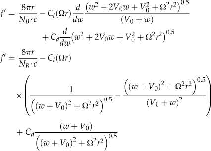
Finally, rewrite by using the effective resultant velocity, VE:
![]() (14-77)
(14-77)
Having defined f(w) and f′(w), we can now determine the root of f, i.e. the value of w that results in f(w) = 0. The value of w is the induced velocity at the blade element at blade station r. Using the Newton-Raphson iterative scheme (mentioned earlier) this would be implemented as follows.
Step 1: Initial Value
Start with an initial value of w, call it w0.
Step 2: Determine the Next w
Calculate the next value of w, call it w1, using the following expression;
![]()
where f(w) is calculated from Equation (14-76) and f′(w) from Equation (14-77).
Step 3: Determine the Difference
Calculate the difference w1 − w0. If this value is larger than, say, 0.01 then go back to Step 1. Otherwise, the value of w is the current value of w1, completing the solution.
EXAMPLE 14-20
Using the spreadsheet of Example 14-18 determine and tabulate the induced velocity, w, for each element. Then, calculate the average w for the propeller and compare it to that from the actuator-disc theory. Also, compare the thrust, torque, and power required to that of Example 14-18.
Solution
A considerable amount of iterative computational labor is required to solve this problem. For this reason, in the interests of space, only a sample calculation, representing the first iteration of the 10th element, can be demonstrated. What will not be demonstrated is the final outcome of a number of such iterations that are necessary to yield the final theoretical value of the induced velocity for that element (denoted by w10). The same process must be repeated for all the other elements that make up the propeller. To complicate things, this initial w10 changes the induced AOA, αi, of the 10th element and, thus, the section lift and drag coefficients, denoted by Cl and Cd. This changes the loading on the propeller, which in turn calls for a new iteration until the propeller loading no longer changes. As a consequence, subsequent iterations of the w on each blade element requires the use of the new values of the Cl and Cd. This procedure has to be repeated a few times until the solution converges to a fixed value of w (or αi) and therefore a final value of the Cl and Cd. This is illustrated in the procedure below. Preliminaries:
| Number of blades | NB = 3 |
| Forward speed | V0 = 270.1 ft/s |
| Angular velocity | Ω = 261.8 rad/s |
| Radial station | r = 1.767 ft (10th element) |
| Blade chord | c = 0.4070 ft |
| Initial value for w | w10 = 1.00 ft/s |
| Initial AOA | α10 = 7.143° |
Step 1: Start the iterative process to compute w10. Begin by calculating a current value for VE from Equation (iii) using the current (or initial) value of w10;
![]()
Step 2: Use Equation (14-76) to calculate the value of the function f(w), noting that Cl(α10) = 0.950 and Cd(α10) = 0.065 are obtained from the curve-fit expression derived in Example 14-18.
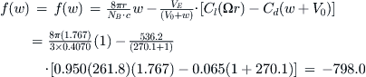
Step 3: Use Equation (14-77) to calculate the derivative of the function f′(w);
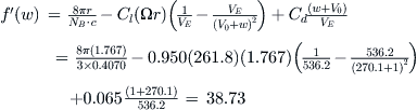
Step 4: Calculate the next value of w10 using the Newton-Raphson iterative algorithm of Appendix E.6.19.
![]()
Step 5: Comparing the original and new w10, we see the difference is 21.60 − 1.00 = 20.60, a comparatively large change between iterations. We want the difference to be much smaller, say 0.0001, before considering our solution fully converged. Before starting the next iteration we must proceed to Step 6 and calculate the induced angle-of-attack, αi 10.
Step 6: Calculate the induced angle-of-attack, αi 10, per Equation (iv).
![]()
This value will be used to recalculate Cl and Cd in the next iteration. The iteration is needed to bypass the problem of circular references in the spreadsheet, and is avoided by copying the induced angles-of-attack and pasting their values (in radians and degrees) into columns 12 and 13, in turn changing the angle of attack in columns 16 and 17 and thus Cl and Cd.
Implementing the methodology in a spreadsheet is relatively easy. Therefore, the next step is to return to Step 1 with the new value of w10 and αi 10 and repeat the calculations, until convergence is achieved. Then go to Step 7. The final value of w10 will be the value of w at blade element number 10.
Note that it is far faster to use the built-in power of Microsoft Excel and create this as functions as shown in Section 14.6.5, Computer code: Determination of the propeller induced velocity, to do these iterations. It returns w without the hassle of having to perform the iteration demonstrated here.
Step 7: Columns 30–36 show how Figure 14-62 shows the values for αi 10 changed in the seven iterations required. The initial value of αi 10 was 0°. After the first iteration αi 10 = 2.269°, and 1.936° after the second and so on. The corresponding induced flow velocity is shown in Figure 14-63. It can be seen that after the 7th iteration, w10 = 18.86 ft/s.
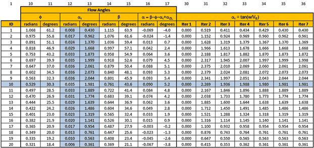
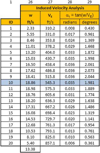
Step 8: The average of w in column 26 in Figure 14-63 is 13.38 ft/s. Let’s compare this value to the induced flow velocity from the actuator disc theory, but this is considered an average value for the entire disc. Using Equation (14-57) we get:

Step 9: Compare T, Q, and P for the propeller, without and with the induced flow:
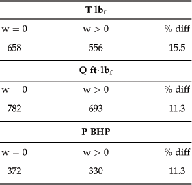
14.6.3 Compressibility Corrections
The local velocity of the blade elements residing near the outboard part of a normally operating propeller is in the high subsonic range. Consequently, these elements should be corrected for compressibility effects. These effects call for corrections of the drag that differ from those for lift. The corrections are applied to the drag and lift coefficients.
Correction of Lift
The lift can be corrected using Prandtl-Glauert, Kárman-Tsien, or Laitone methods (see Section 8.3.6, Compressibility modeling). The latter two must be applied to the pressure coefficients and, thus, require a knowledge of the chordwise distribution of pressure. The first one, Prandtl-Glauert, while simple to apply, becomes gradually inaccurate for airspeeds in excess of M 0.70–0.75.
where
M = helical Mach number (dependent on rotation and forward airspeed per Equation (14-9))
Correction of Drag
The propeller drag at high subsonic speeds must be corrected for skin friction and wave drag. Skin friction can be corrected using the Frankl-Voishel formula of Equation (8-59), where the Mach number at each blade element is evaluated using Equation (14-9). Then, if the Mach number is greater than Mcrit (see Section 8.3.7, The Critical Mach Number, Mcrit) the drag rise at the corresponding Mach number must be determined and applied.
14.6.4 Step-by-step: Prandtl’s Tip and Hub Loss Corrections [14]
The section lift coefficient at the tip of any lifting surface must necessarily go to zero. Unmodified BET ignores this effect and effectively assumes the blade element at the tip generates undiminished lift. This error was recognized by early scientists. Most prominent of those was Ludwig Prandtl (1875–1953), who developed a correction that is easily and conveniently incorporated into the BET. This correction method has been expanded to include corrections at the hub as well (which is another radial where the lift goes to zero). Applying the corrections is a three-step process.
Step 5: Prandtl Correction
Calculate a common correction factor, FP, for Prandtl correction:
![]() (14-83)
(14-83)
The factor FP should vary from 0 at the hub to a value close to 1 over the mid span of the blade, and back to 0 at the tip. This factor is then used by modifying Equations (14-72) through (14-74) as follows:
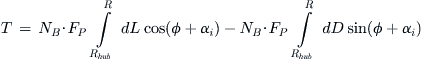

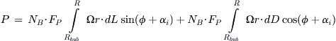
14.6.5 Computer code: Determination of the Propeller Induced Velocity
The solution procedure here was implemented in Microsoft Excel. The program allows the iterative determination of w using the Newton-Raphson algorithm to be written in Visual Basic for Applications (VBA) and is shown below. The function F_of_w calculates the value of f(w) using a number of input variables, V0, Ω, r, NB, c(r), Cd, Cl, and w, using Equation (14-76).
The function InducedVelocity returns the final iterated w. Note that rather than calculating f′(w) using Equation (14-77) it uses a Taylor series finite difference scheme for the derivative (the variable FprimeofX0). It also counts the number of iterations and exits the do-loop if it takes more than 10 interations to converge. The code generally converges in fewer than 10 iterations. This function can be accessed from within Excel by a simple cell reference such as ‘=InducedVelocity(list of input cells)’.

References
1. NACA R-339 Full-Scale Wind-Tunnel Tests with a Series of Propellers of Different Diameters on a Single Fuselage. Weick, Fred E. 1931.
2. Flight International. November 17, 1921; last paragraph p. 761.
3. Stinton D. The Design of the Aeroplane. Collins Professional and Technical Books 1983; p. 304.
4. Beechcraft C90 King Air, Pilot Training Manual. FlightSafety International 2002.
5. In: http://www.faa.gov/regulations_policies/faa_regulations/.
6. AIR1407 Prediction Procedure for Near-Field and Far-Field Propeller Noise. Anonymous 1977.
7. Raymer DP. Aircraft Design: A Conceptual Approach. 4th edn AIAA Eduation Series 2006.
8. TCDS A00009CH Cirrus Design Corporation. Revision. 12/29/2011;18 FAA.
9. Stepniewski WZ, Keys CN. Rotary-Wing Aerodynamics. Dover 1984; p. 46.
10. Massey, Stanford B, Ward-Smith J. Mechanics of Fluids. vol. 1 7th ed. Nelson Thornes 2001.
11. Drzewiecki S. Théorie Générale de L‘Hélice. Gauthiers-Villars et Cie Éditeurs 1920.
12. Stepniewski WZ, Keys CN. Rotary-Wing Aerodynamics. Dover 1984; 94.
13. NACA TR-502 Scale Effect on Clark Y Airfoil Characteristics from NACA Full-Scale Wind-Tunnel Tests. Silverstein, Abe 1935.
14. Glauert H. Airplane Propellers. Aerodynamic Theory In: Durand WF, ed. Berlin: Springer Verlag; 1935; Div. L, Chapter XI.
1Note that a one-bladed propeller usually features a single helical coil shaped like a wood screw. An example of this is David Bushnell’s Turtle submarine from 1776.
2Or hydrodynamic in the case of watercraft.
3For instance see NACA RM-SL53G10, Low-Speed Investigation of the Static Lateral Stability and Control Characteristics of a 1/6-Scale Model of the Republic XF-84H Airplane with the Propeller Operating, for investigation of the type.
4SHP stands for shaft horse-power, a unit of power used for turboprops.
5Broadband noise refers to sound that, by definition, extends over a wide range of frequencies, perhaps even the entire range of audible frequencies.
6The propeller’s Type Certificate Data Sheet P904 69CK, 72CK, 72CC.
7In which the engine components can still rotate.
8If it helps, remember low pitch for low speed and high pitch for high speed.
9The De Havilland DHC-8 DASH 8 is an example of a twin-engine commuter aircraft that has both propellers rotating clockwise as seen from behind. The Fokker F-27 Friendship is an example of a twin-engine commuter that has both propellers rotating counter-clockwise.
10Pilots use the mnemonic: “step on the rudder that’s on the same side as the ball.”
11Pilots use the mnemonic: “dead foot, dead engine.”
12Note that it differs from contra-rotating propellers, which consist of two propellers mounted to the same engine and rotating in the opposite direction. Such propellers are beyond the scope of this book.
13Refers to propellers whose structural core is wood. It is possible to buy wood propellers that have a thin, protective composite (usually fiberglass) coating and sheet-metal leading edges and are marketed as "composite." While true in the literal sense, the structural core of the blades is still wood and, thus, they should not be misclassified as an advanced composite propeller. These wood-composite propellers have thicker tips and trailing edges just like the classic varnished wood blades. Just think: if the composite shield is removed you’ll still have a solid propeller behind it capable of reacting all the applied aerodynamic and inertia loads. If the wooden core is removed you’ll have a thin layer of composite protection, unable to react the same.
14Refers to traditional forged-aluminum blades.
15Refers to typical carbon/epoxy blades with a metal leading edge erosion shield.
16Note that power can be defined as a rate of change of energy, i.e. P = dE/dt.
17Sometimes casually called prop efficiency.
18When the crankshaft is connected to a gear reduction drive the BHP is normally referred to as the shaft horsepower, or SHP. SHP is also used to denote the power of turboprops. In the interests of simplicity, the term BHP can mean either; i.e. the power available at the hub of the propeller.