
Performance – Landing
Abstract
The chapter presents the fundamental relations of the landing phase, including the equation of motion for a landing ground run and its kinematics. Then, several methods to solve the equation of motion are presented. Finally, landing performance data for selected single and multi-engine GA aircraft are tabulated to provide the designer with comparison to own estimation.
Keywords
Approach distance; flare distance; free-roll distance; braking distance; landing over 50 ft; total distance; flare maneuver; ground friction; reference speed; touch-down; braking; and sensitivity
Outline
22.1.1 The Content of this Chapter
22.1.2 Important Segments of the Landing Phase
22.2 Fundamental Relations for the Landing Phase
22.2.1 General Free-body Diagram of the Landing Roll
22.2.2 The Equation of Motion for the Landing Roll
22.2.3 Formulation of Required Aerodynamic Forces
22.2.4 Ground Roll Friction Coefficients
22.2.5 Determination of the Approach Distance, SA
Derivation of Equations (22-5) and (22-6)
22.2.6 Determination of the Flare Distance, SF
22.2.7 Determination of the Free-roll Distance, SFR
22.2.8 Determination of the Braking Distance, SBR
22.2.9 Landing Distance Sensitivity Studies
22.2.10 Computer code: Estimation of Landing Performance
22.1 Introduction
Just as the sections about performance began with the T-O, it is appropriate to end with the landing phase. Figure 22-1 shows an organizational map displaying the landing phase among other members of the performance theory. It is equally important that the designer understands the limitations and sensitivity of this important maneuver as that of the T-O. This section will present the formulation of and the solution of the equation of motion specifically for the landing, and present practical as well as numerical solution methodologies that can be used both for propeller and jet-powered aircraft.
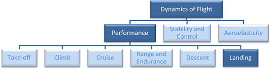
FIGURE 22-1 An organizational map placing performance theory among the disciplines of dynamics of flight, and highlighting the focus of this section: landing performance analysis.
The landing phase is in many ways the inverse of the T-O phase. It begins with the approach to landing in the form of a steady descent. This is followed by a flare maneuver, in which the pilot raises the nose of the aircraft in order to slow it down for a soft touch-down on the runway. The phase terminates with a deceleration from the touch-down airspeed to a complete standstill. The purpose of the analysis methods presented in this section is to determine the total distance the entire maneuver takes.
The landing phase can inflict a serious challenge on aircraft, in particular if its approach speed is high. As the airplane nears the runway it succumbs to ground effect, in which induced drag decreases and lift increases. This may cause the airplane to ‘float’ before it eventually settles on the runway. If its airspeed is high, a significant portion of the runway may be consumed before the airplane can even begin to decelerate to a full stop. Understanding the types and length of runways the airplane is likely to operate from will help size the wing area, choose the landing gear system, and select high-lift and speed-control systems to make it possible to meet the prescribed requirements.
In general, the methods presented here are the industry standard and mirror those presented by a variety of authors, e.g. Perkins and Hage [1], Torenbeek [2], Nicolai [3], Roskam [4], Hale [5], Anderson [6] and many, many others.
22.1.2 Important Segments of the Landing Phase
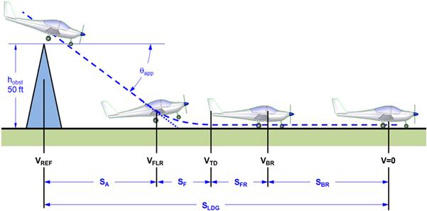
Generally, the landing phase is split into the segments shown in Figure 22-2. The approach distance is measured from the point at which the airplane is 50 ft above ground; the point where the pilot initiates the next maneuver – the flare – by pulling the control wheel (or stick or yoke) in order to raise the nose of the aircraft. This maneuver is required to slow the descent of the airplane in an attempt to help it gently touch down on the runway. The next distance is the flare distance, which extends to the point where the airplane touches down. Then, the airplane typically rolls briefly before the pilot applies the brake system. This distance is referred to as the free-roll distance. Finally, the braking distance accounts for the length of runway required to apply brakes (thrust reversers, drag chute, wheel brakes, etc.) and bring the aircraft to a complete stop.

In short, the purpose of the landing analysis is to estimate the total landing distance by breaking it up into the aforementioned segments and analyzing each of those using simplified physics that pertain primarily to those specific segments. For analysis, the segments are denoted by the nomenclature indicated in Figure 22-3.
Certification requirements for GA aircraft are largely stipulated in 14 CFR Part 23, paragraphs 23.73 through 23.77. Paragraph 23.75 details requirements for the landing distance, shown below:
The designer should be particularly concerned with paragraph 14 CFR 23.77, Balked Landing, as this may inflict serious demands for control surface authority on the airplane.
The specific segments shown in Figure 22-3 are determined in the sections listed in Table 22-1.
TABLE 22-1
Sections Used to Estimate Various Segments of the Landing Run
| Segment Name | Symbol | Section |
| Approach distance | SA | 22.2.5 Determination of the approach distance |
| Flare distance | SF | 22.2.6 Determination of the flare distance |
| Free-roll distance | SFR | 22.2.7 Determination of the free-roll distance |
| Braking distance | SBR | 22.2.8 Determination of the braking distance |
22.2 Fundamental Relations for the Landing Phase
In this section, we will derive the equation of motion for the landing, as well as all fundamental relationships used to evaluate the ground run segment of the landing maneuver. We will consider both conventional and taildragger configurations.
22.2.1 General Free-body Diagram of the Landing Roll
For a free-body diagram of the aircraft during descent refer to Figure 21-2 and for a free-body diagram of the aircraft after touch-down, refer to Figures 17-8 and 17-9, which apply for tricycle and taildragger configurations, respectively. Note that the drag, D, should be modified to reflect the aircraft in its landing configuration and the application of braking devices.
22.2.2 The Equation of Motion for the Landing Roll
The equation of motion for an aircraft during ground roll after touch-down on a perfectly horizontal and flat runway can be estimated from Equation (15-1) with slight modifications. This is simply the inclusion of the effect of braking devices, such as drag chutes, deployed spoilers or speed brakes. The application of mechanical brakes is treated using the ground friction coefficient, μ. Note that the drag coefficient must be that of the aircraft in the landing configuration. Deployed flaps and slats will greatly increase the drag of the aircraft. Additionally, the magnitude of the “acceleration” should always be less than 0 for a deceleration:
where
Dldg = drag in the landing configuration as a function of V, in lbf or N
g = acceleration due to gravity, ft/s2 or m/s2
L = lift of the airplane in the landing configuration as a function of V, in lbf or N
T = thrust (small during landing, but not necessarily negligible), in lbf
W = weight, assumed constant, in lbf
μ = ground friction coefficient (see Table 22-2)
We can also formulate the deceleration of the airplane on a downhill slope, which will increase the total landing distance. This formulation is based on Equation (15-2), but again features minor modifications.
22.2.3 Formulation of Required Aerodynamic Forces
Refer to Section 17.2.4, Formulation of required aerodynamic forces, with the exception of the following:
where
CDi(CL LDG) = induced drag coefficient of aircraft during the landing run after touchdown
αLDG = angle-of-attack of aircraft during the landing run after touchdown
Use the methods of Section 15.5.8, Drag of deployed flaps, to estimate ![]() . Also note that the induced drag must be corrected for ground effect, in particular if the airplane uses flaps or if its attitude is such its ground run AOA is high. Refer to Section 9.5.8, Ground effect for a correction method.
. Also note that the induced drag must be corrected for ground effect, in particular if the airplane uses flaps or if its attitude is such its ground run AOA is high. Refer to Section 9.5.8, Ground effect for a correction method.
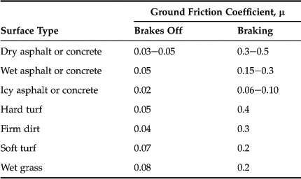
22.2.4 Ground Roll Friction Coefficients
The airplane has to overcome aerodynamic drag and ground friction during the ground roll. The ground friction depends on the weight on wheels and the properties of the ground, which are assessed using the ground roll friction coefficients Table 22-2. This is the same table as Table 17-3, and is merely repeated for convenience.
22.2.5 Determination of the Approach Distance, SA
The geometry of the approach for landing is shown in Figure 22-4. In order to determine the distance from the obstacle to the point where the pilot initiates flare, the approach angle, θapp, and flare height, hF, must be computed. The target approach angle for most airplanes is 3°. For instance, airport approach lights (VASIS or visual approach slope indicator system) give the correct light signal when the airplane is approaching at that descent angle. For other applications, the approach angle can also be calculated using Equations (21-8) or (21-9) for unpowered or powered descents, repeated here for convenience:
However, as stated above, simply assuming θapp = 3° is a good initial assumption. Knowing θapp allows the approach distance, SA, to be estimated by first calculating the flare height, hF, from the following expression:
![]() (22-5)
(22-5)
The airspeeds used in the analysis are listed in Table 22-3 below:
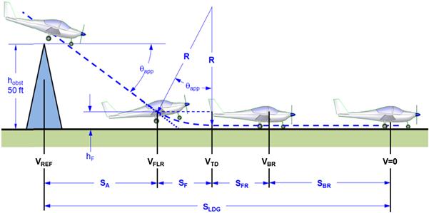
TABLE 22-3
Definition of Important Airspeeds for the Landing Run

aPer 14 CFR Part 23, § 23.73 Reference Landing Approach Speed.
bActual VREF is established per 14 CFR Part 25, § 25.125 Landing.
Derivation of Equations (22-5) and (22-6)
Assume the flare involves slowing down from VREF (= 1.3VS0) to airspeed just above stall, where VS0 is the stalling speed in the landing configuration. Many pilots of light aircraft slow down enough to initiate the audible stall warning of the airplane, reminding us that pilot technique can have great influence on the total landing distance. The aural warning often begins to sound some 5 knots above the stalling speed. This may be less than 10% of the stalling speed. This is further influenced by the ‘floating’ of the airplane in ground effect. For analysis purposes, we must rigorously define the characteristics of the landing maneuver, while at the same time being mindful of the importance of pilot technique. Larger GA aircraft slow down to perhaps 10–15% above stall. Here the airspeed immediately before touchdown will be assumed to be 10% of the stalling speed or VTD = 1.1VS0. This implies an average airspeed of 1.2VS0 during the maneuver and this is used in addition to an assumed lift coefficient of about 0.9CLmax to determine distance traveled as follows:
STEP 1: Average vertical acceleration in terms of load factor.
![]() (22-7)
(22-7)
STEP 2: Using Equation (19-37) (derived in Chapter 19) we calculate the transition radius, R:
![]() (22-8)
(22-8)
where the resulting constant of 0.1512 is applicable to GA aircraft only.
STEP 3: Determine the flare height:
![]() (22-9)
(22-9)
QED
22.2.6 Determination of the Flare Distance, SF
By observation using Figure 22-4, the flare distance, SF, can be determined from:
![]() (22-10)
(22-10)
22.2.7 Determination of the Free-roll Distance, SFR
The free-roll distance is determined in a similar manner to rotation distance in the analysis of the T-O. The airplane is assumed to roll freely for a few seconds only. Thus, the airspeed is assumed constant at VTD (see Figure 22-4), which of course implies that VTD = VBR. Here it is appropriate to assume that small aircraft travel freely for 1 second and large aircraft for 3 seconds. This results in similar equations to those of Section 17.3.4, Determination of Distance during rotation, or:
22.2.8 Determination of the Braking Distance, SBR
The final segment involves the determination of the distance when the pilot begins to apply any braking device until the airplane comes to a complete stop. Braking devices can be conventional mechanical brakes, deployed spoiler, drogue (or drag) chutes, thrust reversers, and so on. For analytical convenience, the deceleration can be considered to consist of the simultaneous contribution of all such braking devices. The scenario in which a drogue chute is deployed, followed by the application of mechanical brakes, or similar complex application of braking devices, requires a numerical integration with respect to time, similar to that of Section 17.3.3, Method 3: Solution using numerical integration. A simpler approach can be based on the method presented in Section 17.3.1, Method 1: General solution of the equation of motion. The approach is applicable to both piston-engine airplanes as well as jets; the only difference lies in how the thrust is calculated. The ratios inside the brackets are evaluated when ![]() , where VBR is the airspeed when the braking is first applied:
, where VBR is the airspeed when the braking is first applied:
![]() (22-13)
(22-13)
Note that the thrust, T, can be either positive or negative (see Table 22-4). It is positive for fixed-pitch or constant-speed propellers, but is negative if reverse thrust is applied. Also note that the negative sign in front of the expression ensures that the distance will be a positive value, since the denominator (the deceleration) will have a negative sign.
TABLE 22-4
Definition of Important Airspeeds for the Landing Run
| Type of Engine | Sign of Thrust | Comment |
| Fixed-pitch propeller | T > 0 | Assume T ≈ 5–7% of static thrust; 5% for cruise propellers and 7% for climb propellers |
| Constant-speed propeller | T > 0 | Assume T ≈ 7% of static thrust |
| Reverse-thrust props – piston | T < 0 | Assume T ≈ −40% of static thrust |
| Reverse-thrust props – turboprop | T < 0 | Assume T ≈ −60% of static thrust |
| Jet – no thrust reverser | T > 0 | Assume T = Tidle |
| Jet – thrust reverser | T < 0 | Assume T ≈ −40% to −60% of static thrust. Can typically only be operated at airspeeds higher than 40–50 KCAS |
The term Dlgd is the drag of the airplane in the landing configuration with braking. This usually implies deployed high-lift devices (flaps and slats), but also spoilers or speed brakes. Typically, speed brakes are deployed (often automatically) as soon as the aircraft touches down and then later are retracted before the airplane comes to a complete stop. A similar scenario holds for the thrust reversers. Equation (22-13) is not applicable to such intermittent use of braking devices. These must be solved using numerical integration as mentioned above.
If the propeller efficiency and engine power at ![]() is known, Equation (22-13) can be rewritten as follows:
is known, Equation (22-13) can be rewritten as follows:
 (22-14)
EXAMPLE 22-1
Determine the landing distance over a 50-ft obstacle and landing run for the SR22 on a standard day at S-L. Consider a runway whose braking conditions are estimated using the ground friction coefficient of μ = 0.3. Assume a 3° glide path (θapp), a landing weight of 3400 lbf, propeller efficiency of 0.45 and idle engine power of 50 BHP at the airspeed ![]() . Furthermore, assume a CD LDG = 0.040 and CL LDG = 1.0. Compare to the POH values of 1141-ft ground roll and 2344 ft over 50 ft.
. Furthermore, assume a CD LDG = 0.040 and CL LDG = 1.0. Compare to the POH values of 1141-ft ground roll and 2344 ft over 50 ft.
Solution
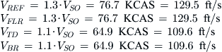
Begin by determining the four airspeeds of interest, VREF, VFLR, VTD, and VBR, based on GA aircraft and noting that the stalling speed in the landing configuration is VS0 = 59 KCAS.
Then, the approach distance must be determined. The flare height, hF, is estimated using Equation (22-5):
![]()
The obstacle height, hobst, for GA aircraft is 50 ft. The distance covered from an altitude of 50 ft to the beginning of the flare is determined using Equation (22-6):
![]()
The distance covered during the flare is given by Equation (22-10):
![]()
The airplane will roll for a brief moment after touch-down before the pilot applies brakes. The distance covered during this time, which for a GA aircraft is considered 1 second, is called the free-roll distance, SFR. It is obtained using Equation (22-11):
![]()
Finally, the braking distance is calculated using Equation (22-14):
![]()
To solve this, it is easiest to calculate the lift and drag separately. Note that the value of CL LDG, given as 0.9, is simply the value at an AOA of 0° (or whatever landing attitude is considered realistic). Note that here this means that with the flaps deflected in the landing setting (for the SR22 this is 32°) it is assumed to equal 0.9.
Inserting these numbers into Equation (22-14), yields:

The total landing distance from 50 ft is thus:
![]()
These numbers deviate as follows from the POH values:
This method is in good agreement with the book values.
22.2.9 Landing Distance Sensitivity Studies
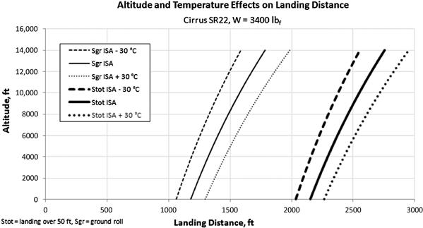
Landing at high elevations and on hot days, when density is much lower than on a standard day at S-L, poses serious challenges to airplane operations. Since the airplane necessarily moves faster with respect to the ground than at lower altitudes, the landing distance increases and the brake energy required to slow down from that higher airspeed is much higher (it depends on the kinetic energy). These effects are corrected through the density and the use of true airspeed.
Using this method, the sensitivity of the landing distance to altitude and temperature is presented in Figure 22-5. The graph plots the estimated landing distance for the SR22 from S-L to 14,000 ft for ±30°C deviations from ISA. It can be seen that at S-L the temperature deviation results in about ±120-ft change in landing over a 50-ft obstacle, when compared to standard day conditions.
22.2.10 Computer code: Estimation of Landing Performance
The following Visual Basic for Applications routine can be used to determine the landing distance for an aircraft. The routine assumes that as long as the obstacle height is larger than zero the entire landing distance will be determined. The simple trick in order to extract the landing ground roll only is to set the obstacle height to zero. This way, the routine works for both evaluations. Note that the routine makes calls to the routine AtmosProperty (see Section A.2.10, COMPUTER CODE A-1: Atmospheric modeling) in order to allow the user to evaluate landing distances at hot and high airports. This is done using the arguments H and deltaISA, where the temperature deviation is that from the standard temperature at that altitude. This code was used with Microsoft Excel to generate the graph of Figure 22-5.
22.3 Database – Landing Performance of Selected Aircraft
Table 22-5 shows the landing run and distance from a 50-ft altitude above ground level. This data is very helpful when evaluating the accuracy of one’s own calculations.


References
1. Perkins CD, Hage RE. Airplane Performance, Stability, and Control. John Wiley & Sons 1949.
2. Torenbeek E. Synthesis of Subsonic Aircraft Design. 3rd edn Delft University Press 1986.
3. Nicolai L. Fundamentals of Aircraft Design. 2nd edn 1984.
4. Roskam J, Lan Chuan-Tau Edward. Airplane Aerodynamics and Performance. DARcorporation 1997.
5. Hale FJ. Aircraft Performance, Selection, and Design. John Wiley & Sons 1984; 137–138.
6. Anderson Jr JD. Aircraft Performance & Design. 1st edn McGraw-Hill 1998.