
Initial Sizing
Abstract
Powerful methods to perform the initial sizing of the airplane are presented. Starting with definition of cost, effectiveness, and cost-effectiveness, the chapter then presents a powerful method, called Constraint Analysis that helps the designer determining the W/S and T/W (or P/W) for the new design such that it will meet all prescribed performance requirements. This is followed by an introduction to various trade studies tools. Trade studies comprise methods that offer powerful approaches for the solution of various engineering problems. This includes carpet plots, design of experiments, and cost function approaches.
Keywords
Design of experiments; carpet plot; constraint analysis; design space; cost function; cost-effectiveness; multi-disciplinary optimization; W/S; T/W; PBHP/W
Outline
3.1.1 The Content of this Chapter
Software for Statistical Analysis and Data Visualization
Software for Multi-disciplinary Optimization
T/W for a Level Constant-velocity Turn
T/W for a Desired Specific Energy Level
T/W for a Desired Rate of Climb
T/W for a Desired T-O Distance
T/W for a Desired Cruise Airspeed
T/W for a Service Ceiling (ROC = 100 fpm or 0.508 m/s)
Derivation of Equations (3-1) and (3-2)
3.2.2 Introduction of Stall Speed Limits into the Constraint Diagram
CLmax for a Desired Stalling Speed
3.3 Introduction to Trade Studies
3.3.1 Step-by-step: Stall Speed – Cruise Speed Carpet Plot
Step 3: Calculate Aerodynamic Properties
Step 4: Tabulate Stall Speeds as a Function of CLmax and Wing Area
Step 5: Calculate and Tabulate Maximum Airspeeds as a Function of Wing Area
Step 6: Tabulate Maximum Airspeeds in Preparation for Plotting
3.1 Introduction
A successful aircraft development program is the consequence of a satisfactory solution to a large number of dissimilar problems. Ideally, we want our airplane to have a low empty weight, good performance, easy handling, a stout light structure, be inexpensive to manufacture and operate, and so on. All of these present different problems to the design process and each require a specific solution. For this reason, the best solution to each individual problem is not necessarily the best solution from a synergistic standpoint.
In fact, the application of such methods is integral to the design process. Designers conduct various trade studies to find the best solution to problems that simultaneously involve a large range of engineering disciplines and project economics. Ultimately, the purpose is to bring to market a useful product that reduces acquisition and operational costs, while improving the performance of the previous technology. Achieving this requires compromise and balance. Airplanes designed with only one discipline in mind will unlikely satisfy other requirements.
A classic example of this is the sizing of the wing area. A large wing area leads to a lower stalling speed; if the design problem is simply “low stalling speed” or a “lot of fuel capacity,” then a large wing area is an obvious solution. However, if speed and efficiency are a goal too, a large wing area is detrimental. It increases drag and structural weight and ignoring these will result in a poor design, no matter how low the stalling speed.
A correct sizing of an airplane depends on a large number of very important variables such as those discussed in Section 1.1.2, Important elements of a new aircraft design. A clearly stated mission plays a paramount role in this respect and allows the sizing to be accomplished using mathematical tools. This section presents a few optimization methods that focus on the external geometry of the airplane. Of these, the most prominent is the so-called constraint analysis. The method is used to determine the appropriate wing area and engine power (or thrust) for a new design, based on a number of performance requirements. The section will also introduce a method called design of experiments (DOE), carpet plots, and a simple discussion of cost functions.
3.1.1 The Content of this Chapter
• Section 3.2 presents a powerful method, called constraint analysis, that helps the designer determine the wing sizing (W/S) and thrust-to-weight ratio (T/W or P/W) for the new design, so that it will meet all prescribed performance requirements.
• Section 3.3 presents several trade study methods, which are powerful tools for the solution of various engineering problems.
3.1.2 Fundamental Concepts
Among a number of concepts frequently brought up in trade studies are cost, effectiveness, and cost-effectiveness. While these concepts apply to a large number of topics, in aviation they usually apply to operational and performance efficiency of the aircraft. In this context, operational efficiency refers to the cost associated with acquiring, maintaining, and using (operating) the vehicle. The operational efficiency puts a serious constraint on unconventional aircraft configurations. Historically, unconventional aircraft do not enjoy great market acceptance (they are unconventional after all). As demonstrated in Section 2.2.2, Development cost of a GA aircraft – the Eastlake model, the cost of acquisition is directly related to the number of units delivered. It is a serious drawback for such designs that they lack the operational experience of their “conventional” competitor aircraft.
In its simplest terms, performance efficiency refers to the magnitude of the maximum lift-to-drag ratio. As is evident from the formulation of the performance chapters of this book, this ratio has a profound effect on key performance parameters such as range and endurance. High fuel costs make this figure of merit even more important than before. This implies that the aircraft designer should strive to develop an aircraft that is aerodynamically sleek and one that requires low engine power for cruise.
Cost
The cost of an aircraft includes the cost of the resources needed to design, manufacture, and operate it. Resources include engineers, technicians, and administrative staff; as well as contractors, materials, office and manufacturing facilities; and specialized equipment such as wind tunnels. Cost is most often represented using monetary units such as dollars. Trade studies always try to minimize cost.
Effectiveness
The effectiveness of an aircraft refers to a quantitative measure of how well the aircraft achieves its mission. This is highly dependent upon its performance. For instance, consider an aircraft designed for a long-distance flight. Its effectiveness can be defined as the ratio of the actual range to the intended range. Effectiveness sells. Trade studies always try to maximize effectiveness.
Cost-effectiveness
The cost-effectiveness of a system combines both the cost and the effectiveness of the system in the context of its objectives. While it may be necessary to measure either or both of those in terms of several numbers, it is sometimes possible to combine the components into a meaningful, single-valued objective function for use in design optimization. Even without knowing how to relate effectiveness to cost, designs that have lower cost and higher effectiveness are always preferred.
Usually the hardest part of any trade study is to formulate the various effects. Some examples of how this can be done will be shown in this text. Three types of trade studies are discussed: constraint analysis, graphical trade study, and Multi-Disciplinary Optimization (MDO). The reader should know that such studies are a field of specialization within engineering and, therefore, only an elementary introduction is given here.
3.1.3 Software Tools
A large number of software packages have emerged that provide substantial help in harnessing the computational power of the modern computer. A number of sophisticated data visualization packages are available, as well as software that make running MDO easy. Detailed description of such software, other than a brief explanation of what such packages do, is beyond the scope of this text.
Software for Statistical Analysis and Data Visualization
A large number of software packages capable of presenting statistical analyses results using powerful visualization are available, both as commercial packages and as freeware.1 Some software is ideal for work involving design of experiment (see Section 3.3.2, Design of experiments), for instance JMP Software (www.jmp.com). Others include statistical analyses with other capabilities, such as Mathematica (www.wolfram.com/mathematica), Maple (www.maplesoft.com), and MATLAB (www.mathworks.com).
Software for Multi-disciplinary Optimization
A number of powerful packages intended for MDO are also available.2 Many such software packages allow the user to connect multiple unrelated external software solutions together and run them from a central hub (e.g. AIMMS PRO from www.aimms.com, PHX ModelCenter from www.phoenix-int.com, and HEEDS MDO from www.redcedartech.com/products/heeds_mdo). For instance, it is possible to connect Microsoft Excel analysis to some unrelated analyses (e.g. software and dynamic link libraries written using FORTRAN, C, C++, Visual Basic, etc.) that could be running as an MS-DOS or Windows process. This is done by “telling” the program what the input and output variables mean and how they relate to one another. Such software will then often rewrite the input files, run the associated external software through a batch operation, read the resulting output file, and use the data as a part of the overall optimization. The power of such software is realized when companies can put existing “in-house” programs to use with very limited effort.
3.2 Constraint Analysis
One of the first tasks in any new aircraft design is to perform a constraint analysis using a special graph called a constraint analysis graph. The primary advantage of this graph is that it can be used to assess the required wing area and power plant for the design, such that it will meet all performance requirements.
Constraint analysis is used to assess the relative significance of performance constraints on the design. This is done by plotting the constraints on a special two-dimensional graph called the design space (see Figure 3-1). Commonly the two axes represent characteristics such as (y-axis) thrust-to-weight ratio (T/W) and (x-axis) wing loading (W/S). The graph is then read by noting that any combinations of W/S and T/W that are above the constraint curves will result in a design that meets those requirements. The white-colored region in the figure is the domain of acceptable solutions. The shaded region represents unacceptable solutions. For instance, Design A would meet the T-O run and climb requirements, design C would meet none, and design E all but the climb. Design F meets all requirements. The graph allows the designer to see at a glance the combination of W/S and T/W that allows the requirements to be met.
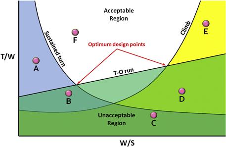
FIGURE 3-1 Typical design space. Only a combination of T/W and W/S that lie in the white (acceptable) region constitute viable design. Here F is the only viable design, albeit not optimal.
The graph also features optimum design points, at which the least amount of power or thrust is required to meet all applicable requirements. Of the two points shown, the true optimum is the one that offers the lower W/S and T/W. This point results in minimum power required and this usually means a power plant that is less expensive to acquire and operate. The designer should also consider the impact of the W/S on the stalling speed of the aircraft. For instance, the 14 CFR Part 23 stall speed maximum is 61 KCAS3 or 45 KCAS for Light Sport Aircraft (LSA).4 Section 3.2.2, Introduction of stall speed limits into the constraint diagram, will introduce how to incorporate this important limit into the constraint diagram.
The key to creating a constraint graph is the conversion of applicable formulas into a form such that T/W is a function of W/S. Transcendental functions have to be solved iteratively. The optimum points indicate where the design can be accomplished at a minimum cost (less power required usually means smaller, less expensive power plant).
3.2.1 General Methodology
The general methodology of constraint analysis requires some performance characteristics of interests to be described using mathematical expressions. In order to be useful, the expressions must be converted into the proper format that allows them to be evaluated. This section focuses on converting the performance characteristics into the form T/W = f(W/S). However, the reader should be mindful that other criteria besides T/W and W/S may be considered. For the design of GA aircraft, the following basic formulation is very practical. They are all based on the simplified drag model (See Chapter 15, Aircraft drag analysis), so the designer should expect some deviations from a more sophisticated analysis. This is not important, however, because little is known about the design when they are used anyway – they represent some of the earliest steps in the design process.
T/W for a Level Constant-velocity Turn
The following expression is used to determine the T/W ratio required to maintain a specific banking load factor (n) at a specific airspeed and altitude, without losing altitude. For instance, consider a project where the design is required to maintain a 45° bank angle at a given airspeed. The first step would be to convert the angle into a load factor, n, using Equation (19-36). Then, the expression would be used to determine the required T/W as a function of W/S.
![]() (3-1)
(3-1)
where
CDmin = minimum drag coefficient
k = lift-induced drag constant
q = dynamic pressure at the selected airspeed and altitude (lbf/ft² or N/m²)
Note that Equation (3-1) corresponds to specific energy density PS = 0 (see Section 19.3.3, Energy State).
T/W for a Desired Specific Energy Level
Sometimes it is of importance to evaluate the T/W for a specific energy level other than PS = 0, as was done above. The following expression is used for this purpose. For instance, consider a project where the design is required to possess a specific energy level amounting to 20 ft/s at a given load factor, airspeed, and altitude. Such an evaluation could be used for the design of an aerobatic airplane, for which the capability of a rival aircraft might be known and used as a baseline.
![]() (3-2)
(3-2)
where
T/W for a Desired Rate of Climb
The following expression is used to determine the T/W required to achieve a given rate of climb. An example of its use would be the extraction of T/W for a design required to climb at 2000 fpm at S-L or 1000 fpm at 10,000 ft.
![]() (3-3)
(3-3)
where
Note that ideally the airspeed, V, should be an estimate of the best rate-of-climb airspeed (VY – see Section 18.3, General climb analysis methods). Since this requires far more information than typically available when this tool is used, resort to historical data by using VY for comparable aircraft. However, it may still be possible to estimate a reasonable VY for propeller aircraft using Equation (18-27).
T/W for a Desired T-O Distance
The following expression is used to determine the T/W required to achieve a given ground run distance during T-O. An example of its use would be the extraction of T/W for a design required to have a ground run no longer than 1000 ft.
![]() (3-4)
(3-4)
where
T/W for a Desired Cruise Airspeed
The following expression is used to determine the T/W required to achieve a given cruising speed at a desired altitude. An example of its use would be the extraction of T/W for a design required to cruise at 250 KTAS at 8000 ft.
![]() (3-5)
(3-5)
where
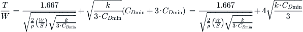
T/W for a Service Ceiling (ROC = 100 fpm or 0.508 m/s)
The following expression is used to determine the T/W required to achieve a given service ceiling, assuming it is where the best rate-of-climb of the airplane has dropped to 100 fpm. An example of its use would be the extraction of T/W for a design required to have a service ceiling of 25,000 ft.
 (3-6)
(3-6)
where
ρ = air density at the desired altitude.
VV = rate-of-climb = 1.667 ft/s if using the UK-system and 0.508 m/s if using the SI-system
Note that service ceiling implies VY (the best rate-of-climb airspeed), as this yields the highest possible value. This is particularly important to keep in mind when converting the T/W to thrust and then to power for propeller aircraft (and as is demonstrated later). For this reason, VY should be estimated, for instance using Equation (18-27) or other suitable techniques.
Additional Notes
(1) Note that when constructing constraint diagrams for propeller aircraft, the analysis is complicated by having to convert the thrust-to-weight ratio to P/W. Such diagrams are far more convenient for propeller-powered aircraft because conventional piston and turboprop engines are rated in terms of horsepower. The conversion is accomplished using Equation (14.38), repeated here for convenience:
![]() (14.38)
(14.38)
(2) Normalization of thrust and power: Since engine thrust or power depends on altitude, a proper comparison requires a transfer of all altitude characteristics to S-L. This can be accomplished for piston-engine power using the Gagg-Ferrar model, presented in Equation (7-16). For gas turbines the method of Mattingly et al., presented in Section 7.2, The properties of selected engine types, can be used. Alternatively, if the airplane is powered with a gas turbine, the designer may have access to an “engine deck” which is software written by the engine manufacturer that allows the thrust (or SHP) at a given altitude, airspeed, and other operational parameters to be extracted. Using such software, the designer should make sure the engine can generate the required thrust or SHP in the corresponding conditions.
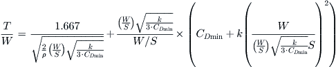
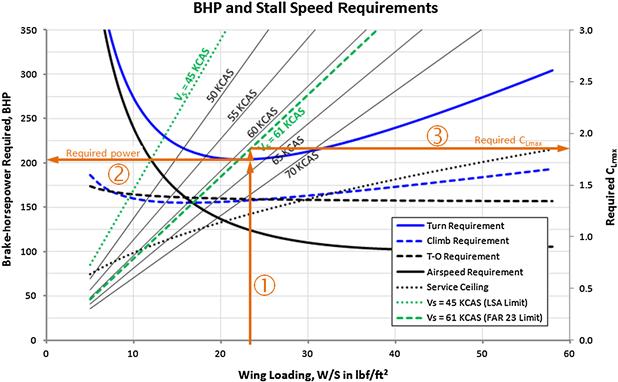
A case in point is the constraint diagrams seen in Figure 3-2 and Figure 3-3 for Example 3-1, developed in conjunction with the constraint curves superimposed on the design space. The fact is that some are plotted at S-L conditions, while others represent higher altitudes. Consider the curve representing the service ceiling in Figure 3-3. At W/S = 30 lbf/ft² this requirement calls for approximately 160 BHP at 20000 ft. The point is that, using the Gagg and Ferrar model, this means the engine must be capable of producing at least 340 BHP at S-L at that wing loading. Therefore, we say that the higher horsepower number (340 BHP) has been normalized to S-L conditions. Note that Figure 3-4 shows all the requirements presented in the example normalized in this fashion.
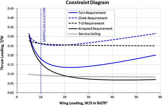

FIGURE 3-3 Plotting required BHP for the various requirements. This graph displays the T/W ratios of Figure 3-2 converted to corresponding power in BHP at each altitude.
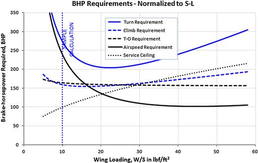
FIGURE 3-4 Required power in BHP for the various requirements normalized to S-L conditions. This graph makes it possible to realistically select an engine for the aircraft.
(3) Note that the dynamic pressure, q, is always calculated at the specific condition for which it refers. This way, the following rules apply to q:
Equation (3-1): q is calculated at the turning airspeed and the associated altitude.
Equation (3-3): q is calculated at the climb airspeed and the associated altitude.
Equation (3-4): q is calculated at ![]() in accordance with Section 17.3.1, METHOD 1: General solution of the equation of motion and the associated altitude.
in accordance with Section 17.3.1, METHOD 1: General solution of the equation of motion and the associated altitude.
Equation (3-5): q is calculated at the desired cruising speed and the associated altitude.
Equation (3-6): ρ is at the desired service ceiling.
(4) One of the problems encountered at this stage of the design is that the geometry of the airplane is largely unknown. For that reason, one does not know important parameters such as CDmin, CDTO, CLTO, and k. To resolve this issue, the designer must look to existing aircraft in the same class as the one being designed and try to estimate them. Table 3-1 is intended to give the designer a range of typical values, in lieu of such a study. Also, consider Table 15-18, which lists CDmin for a number of selected aircraft.

Derivation of Equations (3-1) and (3-2)
Consider Equation (19-40) for thrust required in a sustained turn at a load factor n, here repeated for convenience (ignoring the trim drag):
![]()
This equation can be put into the desired form by dividing both sides by W (simplifying TREQ by writing T):
![]()
Dividing through by W/S yields Equation (3-1). Note that this formulation features the simplified drag model (see Chapter 15, Aircraft Drag Analysis, in particular Equation (15-5)).
To derive Equation (3-2) we consider the case where there is more thrust available than the required thrust, TREQ. Calling this thrust TAVAIL, we can write this as the thrust required plus additional thrust, ΔT, i.e.:
![]()
Then, insert Equation (3-1) and note that since the power associated with ΔT is ![]() , we can write:
, we can write:
![]()
Then, multiply the additional term by 1 or W/W and note that PS = ΔP/W. This comes from the fact that ROC is power divided by weight (see Chapter 18, Performance – Climb). Therefore, we get:
![]()
Then dividing both sides of the equal sign by W similar to what was done for Equation (3-1) yields Equation (3-2).
QED
Derivation of Equation (3-3)
Consider Equation (18-18) for Rate-of-climb, also repeated for convenience:
![]()
Assuming that small angle relations hold, cos θ ∼ 1, we write:
![]()
Solving for T/W yields Equation (3-3).
QED
Derivation of Equation (3-4)
Assuming the ground run to start from rest, the kinematic relations between acceleration, speed, and distance can be written as:
![]()
Where a is the average acceleration during the T-O run, calculated at VLOF/√2 using Equation (17-4):
![]()
Inserting into the expression for SG this leads to:
![]()
Solving for T/W by algebraic manipulations, this leads to:
![]()
Writing this in terms of T/W to yield a convenient form for use in the design space will give Equation (3-4).
Note that the argument for the equation is effectively ![]() (and not VLOF), as this is used to calculate the acceleretion. Therefore, when extracting power for a propeller powered aircraft, use
(and not VLOF), as this is used to calculate the acceleretion. Therefore, when extracting power for a propeller powered aircraft, use ![]() , where ηp is the propeller efficiency at
, where ηp is the propeller efficiency at ![]() .
.
QED
Derivation of Equation (3-5)
During cruise we may assume thrust to equal drag. Therefore, we can write:
![]()
Expand the above expression and insert the definition for the lift coefficient, ![]()
![]()
Manipulate algebraically by isolating the term W/S:
![]()
Divide through by the weight W and manipulate:
![]()
Rearrange in terms of W/S:
![]()
Since we define the dynamic pressure as q = ½ρV² and the lift-induced drag constant as k = 1/(π·AR·e), these can be inserted into the above expression to yield Equation (3-5).
QED
Derivation of Equation (3-6)
It is assumed that the service ceiling is where the best rate of climb has dropped to 100 fpm. Therefore, using Equation (18-17), it is possible to write:
![]()
Assuming the simplified drag model, this can be rewritten as follows:
![]() (i)
(i)
Noting that using the simplified drag model the best rate-of-climb airspeed for a propeller aircraft is given by:
![]()
Therefore, the dynamic pressure is given by:
![]()
Inserting both of these into Equation (i), yields:
Finally this yields:
QED
EXAMPLE 3-1
A single piston-engine propeller airplane is being designed to meet the following requirements:
(1) Design gross weight shall be 2000 lbf.
(2) It must sustain a 2g constant velocity turn while cruising at 150 KTAS at 8000 ft.
(3) It must be capable of climbing at least 1500 fpm at 80 KCAS at S-L.
(4) It must be capable of operating from short runways in which the ground run is no greater than 900 ft and liftoff speed of 65 KCAS at design gross weight.
(5) It must be capable of a cruising speed of at least 150 KTAS at 8000 ft.
(6) It must be capable of a service ceiling of at least 20,000 ft.
The designer’s initial target is a minimum drag coefficient of 0.025 and an aspect ratio of 9. Furthermore, it is assumed the ground friction coefficient for the T-O requirement is 0.04, the T-O lift and drag coefficients are CL TO = 0.5 and CD TO = 0.04, respectively. Plot a constraint diagram for the design for these requirements in terms of W/S and T/W for values of W/S ranging from 5 to 58 lbf/ft². Then determine the required wing area and horsepower for the airplane if its propeller efficiency is 0.80 (assume it is for all flight conditions, even though this would not hold for real propeller aircraft).
Solution
Step 1: Calculate span efficiency per Section 9.5.14, Estimation of Oswald’s Span Efficiency, here using Method 1:
![]()
Step 2: Calculate the lift-induced drag constant, k, per Equation (15-7):
![]()
Step 3: Calculate the T/W per Equation (3-1). Here, only a sample value of the T/W will be calculated, using W/S = 10 lbf/ft². Then a number of values were calculated using Microsoft Excel and plotted in Figure 3-2. Begin by computing the dynamic pressure at 8000 ft:
![]()
Then calculate the dynamic pressure:
![]()
Then calculate the T/W, say for a sample value of W/S = 10 lbf/ft²:
![]()
Step 4: Calculate the T/W per Equation (3-2). Here, again, only a sample value will be calculated. Begin by noting that the ROC amounts to 1500 fpm/(60 s/min) = 25 ft/s and 80 KCAS at S-L amounts to 135.0 ft/s. First, calculate the dynamic pressure:
![]()
Again, let’s use a sample value of W/S = 10 lbf/ft² to get the following value of T/W:
![]()
Step 5: Calculate the T/W per Equation (3-4). Here we must first determine realistic values for the lift and drag coefficients during the T-O run. Start by calculating the dynamic pressure at V = VLOF/√2:
![]()
Therefore, for the sample value of W/S = 10 lbf/ft², recalling that μ = 0.04, CL TO = 0.5, and CD TO = 0.04, we get the following value of T/W:

Step 6: Calculate the T/W per Equation (3-5), using the ρ and q calculated in Step 3. Then calculate the T/W for the sample value of W/S = 10 lbf/ft² as follows:
![]()
Step 7: Begin by computing the dynamic pressure at 20,000 ft:
![]()
Calculate T/W for the service ceiling using Equation (3-6):
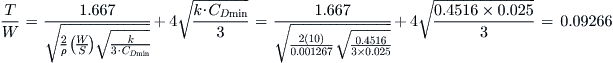
Step 8: By computing the values of T/W for a number of values of W/S we can plot the results as shown in Figure 3-2, where this is done for W/S ranging from 5 to 58. Note that the region above the curves is the acceptable region.
Step 9: Since T/W varies with W/S, pick a token value of W/S to use in a sample calculation in which BHP and wing area are extracted. First, considering the sample W/S = 10 lbf/ft² the weight requirement of 2000 lbf will call for a propeller thrust of 2000 × 0.1799 = 360 lbf to be generated while turning with a 2g loading at 150 KTAS at 8000 ft. Using Equation (14.38) we determine that the engine horsepower at that altitude must be at least:
![]()
This, of course, means that the engine must have a higher rating than 207 BHP, because this is what is needed at 8000 ft. Using the Gagg and Ferrar model (see Equation (7-16)), we can estimate what the S-L rating must be:
![]()
This shows that in order to generate 207 BHP at 8000 ft, the engine will have to be rated at least 273 BHP at S-L.
Similarly, the required wing area can now be obtained from the wing loading. For the above sample of W/S = 10 lbf/ft², the wing area must be S = W/(W/S) = 2000/(10) = 200 ft². Compared to modern airplanes both BHP and S are much larger than the norm for a gross weight of 2000 lbf. Clearly we picked a value of W/S that is not representative of aircraft currently in production. Let us calculate the value of BHP for the range of W/S for all the requirements and find out if anything else can be learned. This has been done in the graph in Figure 3-3.
Figure 3-4 shows this graph normalized. It can be seen that the curves for the turn, airspeed, and service ceiling requirements are shifted upward when compared to Figure 3-3. It is evident that the minimum T/W for the turn requirement occurs when W/S ≈ 22.5 lbf/ft². The resulting airplane will only require around 205 BHP to meet all requirements. This wing loading can be used to establish the required wing area. Doing so, we get the following requirement for the wing area: S = 2000/(22.5) = 89 ft². Should this aircraft be certified under FAR 23 (which requires a maximum stall speed of 61 KCAS) the design will require a maximum lift coefficient of:
![]()
This calls for a simple high lift system to meet the 61 KCAS stall requirement. It will also allow the pilot to perform some steep approaches for landing.
3.2.2 Introduction of Stall Speed Limits into the Constraint Diagram
It is very important to consider stall speed limitations imposed by the regulatory authorities when constructing the constraint diagram. Otherwise, it is possible to inadvertently select a combination of W/S and T/W that, while meeting all other requirements, results in a stalling speed that is too high. It is strongly recommended that the stalling speed is incorporated into the constraint diagram as shown in Figure 3-5. This is accomplished by plotting isobars for selected stalling speeds using a second vertical axis. To do this, the maximum lift coefficient for a given stalling speed is plotted as a function of the wing loading as explained below.
CLmax for a Desired Stalling Speed
For this purpose, the maximum lift coefficient can be considered a function of the wing loading, W/S, for a constant dynamic pressure, qstall, using the expression below:
![]() (3-7)
(3-7)
In using this technique, a target stalling speed is selected. Then, the dynamic pressure, qstall, is determined, after which the maximum lift coefficient is calculated for a range of wing loadings, W/S. It is preferable to repeat this for a number of stalling speeds, say, 5 KCAS apart. Then, these are superimposed on the constraint diagram as isobars using a secondary vertical axis for the CLmax. Figure 3-5 shows this added to Figure 3-3 of Example 3-1. In the example, W/S = 22.5 lbf/ft² was shown to be an optimum. To use this information, consider that we are interested in evaluating the CLmax required for the airplane to stall at VS = 61 KCAS. Following arrow ![]() we move from the horizontal axis to the optimum point and then continue along arrow
we move from the horizontal axis to the optimum point and then continue along arrow ![]() to read about 205 BHP from the left vertical axis. Then, we go back to the optimum point and move to the diagonal isobar labeled ‘Vs = 61 KCAS (FAR 23 Limit).’ Then move horizontally along arrow
to read about 205 BHP from the left vertical axis. Then, we go back to the optimum point and move to the diagonal isobar labeled ‘Vs = 61 KCAS (FAR 23 Limit).’ Then move horizontally along arrow ![]() until the right vertical axis is intersected. There we can read that a CLmax of about 1.78 is required to meet that restriction – something easily accomplished with a simple high-lift system.
until the right vertical axis is intersected. There we can read that a CLmax of about 1.78 is required to meet that restriction – something easily accomplished with a simple high-lift system.
Derivation of Equation (3-7)
The expression is simply obtained from the standard equation for lift, ![]() . At stall we may write:
. At stall we may write:
![]()
QED
3.3 Introduction to Trade Studies
The term trade study (aka trade-off) refers to various methods whose purpose is to identify the most balanced technical solution among a set of proposed viable solutions. A good understanding of such methods is essential for the design engineer and they have a lot of power to offer. For instance, consider the problem of determining a suitable wing area for an aircraft. A large wing area will generally bring down the stalling speed, which is good. However, it will also increase drag and structural weight, which makes the airplane less efficient, which is not good. The three characteristics (lift, drag, and weight) are counterproductive. The designer must eventually weigh the importance of each and make a suitable compromise, which is reflected in the selected wing area. Such tasks are most easily accomplished using trade studies of the nature presented below.
3.3.1 Step-by-step: Stall Speed – Cruise Speed Carpet Plot
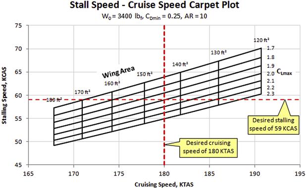
The first method is the preparation of a stall speed – cruise speed carpet plot, which is intended to help the designer select a wing area such that both desired stalling and cruising speed targets can be met. It requires a number of key parameters to be known, unlike the constraint diagram, which requires much less initial knowledge. This renders the method a tool to use after the constraint diagram has been prepared. As such, it is ideal when considering the modification (growth) of existing airplane types.
The creation of the carpet plot appears complicated at first, but in fact it is not, as long as the following steps are followed. The presentation below applies to a propeller powered aircraft and for clarity it will use actual numbers that are similar to the Cirrus SR22, as we pretend we are designing a similar aircraft. This is done because the consequent comparison gives a deeper insight into the usefulness of this method. Finally, note that the method presented uses Microsoft’s Excel spreadsheet program for the analysis.
Step 1: Preliminary Data
Establish design parameters similar to what is shown in Table 3-2.

Note that it is prudent to aim at a stalling speed approximately 2 knots below the 14 CFR Part 23 minimum of 61 KCAS. This is why 59 KCAS is entered as a “desired” number. Also, looking at the competition, it is prudent to aim for at least 180 KTAS at 8000 ft.
Step 2: Decide Plot Limits
Decide the range and steps of maximum lift coefficient, CLmax, to analyze. Here we will pick 1.7 ≤ CLmax ≤ 2.3 with seven steps, of which the magnitude of each is 0.1.
Decide the range of wing areas, S, using the same number of steps as for the CLmax. Similarly, we will pick 120 ≤ S ≤ 180 ft², also with seven steps, each being 10 ft² in magnitude.
Step 3: Calculate Aerodynamic Properties
Calculate the parameters shown in Table 3-3. Note that the density is calculated using Equation (16-18) or (16-19), Oswald’s span efficiency is calculated using Equations (9-89), (9-91), or (9-92), and power at altitude is calculated using Equation (7-16):

Step 4: Tabulate Stall Speeds as a Function of CLmax and Wing Area
Prepare a table of stalling speeds similar to the one shown in Table 3-4 below. The stalling speed in the body of the table is calculated using Equation (19-7) at S-L. Note that the calculated stalling speeds are in terms of ft/s and are converted to KCAS by dividing by the factor 1.688 knots/(ft/s). For instance, using S = 150 ft² and CLmax = 2.0 gives a stalling speed of 97.9 ft/s, which when converted equals 58 KCAS.

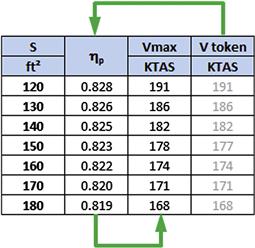
Step 5: Calculate and Tabulate Maximum Airspeeds as a Function of Wing Area
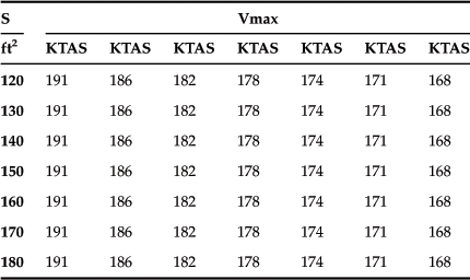
Having completed tabulating the stalling speeds, next calculate the maximum airspeed that corresponds to the range of wing areas selected (here 120 to 180 ft²). It is imperative to realize that this can be accomplished in several ways. Here, methods that use the Visual Basic for Applications functions that have already been developed in this book are picked. For this exercise, two of them will be used; Section 14.5.4, COMPUTER CODE: Estimation of propeller efficiency using the momentum theorem and Section 19.2.14, COMPUTER CODE: Determining maximum level airspeed, Vmax, for a propeller aircraft. They are used together to create a table similar to Table 3-5. Note that the two arrows display important relationships that must be kept in mind when preparing the spreadsheet in order to prevent a circular error from occurring in Excel. The rightmost column labeled V token contains airspeeds that are only used with the function PropEfficiency(BHP, V, H, Dp, Nv). These are actually entered manually and iteratively until they are as close as possible to Vmax – a nuisance step, but necessary to avoid circular error. The PropEfficiency function is used to calculate the propeller efficiency in the column labeled ηp. This is done assuming a viscous profile efficiency, Nv, of 0.85 (see the computer code of Section 14.5.4 for details). Then, the airspeed in the column labeled Vmax uses this value as an argument when using the function Vmax_Prop(S, k, CDmin, W, rho, BHP, eta). If PropEfficiency refers to Vmax directly, a circular error will occur.
Step 6: Tabulate Maximum Airspeeds in Preparation for Plotting
Next prepare a table similar to Table 3-6. This table and those from previous steps will be used to prepare the carpet plot in the next step. Note that in the table below, the airspeeds are repeated, here seven times. This is necessary to create the carpet plot, as will become evident in the next step.
Step 7: Create Carpet Plot
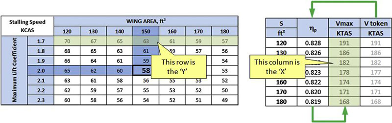
In this step, the carpet plot shown in Figure 3-6 will be created. This involves using the specific rows and columns of Tables 3-4 and 3-5 as shown in Table 3-7 below. To plot the curves with the shallow slope, plot the rows and columns indicated by the shading below. Note how the X and Y values are selected. The table from Step 5 corresponds to X-values and the one from Step 4 is used for Y-values.
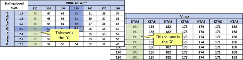
Similarly, the vertical lines are plotted using the scheme shown in Table 3-8. The table in Step 6 is used for the X-values and the one in Step 4 is used for the Y-values.
Once the carpet plot is complete (see Figure 3-6), it is time to interpret it. Considering the vertical lines first, it can be seen that the greater the wing area the slower will be the cruising speed. This way, should the desired CDmin of 0.025 indeed be realized, a 180 ft² wing would result in a cruising speed of 167 KTAS, while a 120 ft² wing would yield 191 KTAS. The analysis performed here does not account for a larger CDmin for the larger wing, but this can easily be included by performing drag analysis.
Continuing with the 120 ft² wing, it can be seen that if it featured a high-lift system capable of generating a CLmax = 2.3, it would have a stalling speed of 60 KCAS. However, if a very simple flap system was employed and it only achieved a CLmax = 1.7, it would stall at 70 KCAS. In either case, it would bust the desired stalling speed of 59 KCAS.
The desired stalling and cruising speeds have been superimposed on the graph. Where the two lines intersect it can be seen that a wing area close to 145 ft² and a high-lift system that generates a CLmax ≈ 2.0 should achieve both target airspeeds. Interestingly, this is precisely what the SR22 features, except that its POH cruising speed at 8000 ft and 78% power is 183 KTAS. This lends great support to the value of this method.
3.3.2 Design of Experiments
Design of experiments (DOE) is a method used to determine which variable(s) from a collection from variables is the most effective contributor to some process. The method is best explained using an example.
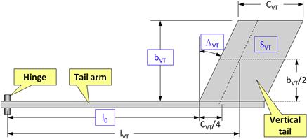
Consider the development of a vertical tail (VT) for some airplane and that we are interested in understanding what properties contribute to its directional stability derivative, Cnβ. To keep things manageable we will analyze the simple constant-chord VT configuration shown in Figure 3-7. The tail is mounted to the hinged tail arm, which allows it to rotate freely, and we can assume the hinge represents the location of the airplane’s center of gravity. Aerodynamic theory dictates that the derivative is affected by the tail arm (lVT), tail planform area (SVT), tail span (bVT), and leading edge sweep (ΛVT). Other contributions, such as that of taper ratio or airfoil type, will be ignored.
The following question can now be asked: Which of the above variables affect the value of the Cnβ the most? For instance, if any of the variables change by, say, 10% from its initial value, which will change Cnβ the most? The answer is important because if we want to change Cnβ, the result simply tells us where to focus our effort.
Before these questions can be answered, the appropriate formulation must be developed. First, the yawing moment, CN, is the product of the lift force acting on the tail, LVT, and its distance from the hinge or tail arm, denoted by lVT:
where
Then, the directional stability, Cnβ, at low yaw angles can be approximated from:
The tail arm, lVT, is based on the dimensions in Figure 3-7 and is calculated from (see the dimensions in the figure):
where
In this analysis, it is better to use the term l0 to control the length of the tail arm. The lift curve slope of the tail, ![]() , can be calculated using Equation (9-57), but this is directly dependent on ΛVT since the configuration features a constant-chord. By varying each of the four variables (l0, bVT, SVT, and ΛVT) over a range of 10%, using some representative numbers for the variables q, S, and b, the graphs of Figure 3-8 were created. The results will now be discussed.
, can be calculated using Equation (9-57), but this is directly dependent on ΛVT since the configuration features a constant-chord. By varying each of the four variables (l0, bVT, SVT, and ΛVT) over a range of 10%, using some representative numbers for the variables q, S, and b, the graphs of Figure 3-8 were created. The results will now be discussed.
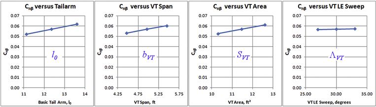
When a specific variable is varied over a range of 10% of its baseline magnitude this simply means that lower and upper bound values are determined and the Cnβ is calculated for each. For instance, consider the VT span, bVT. The lower bound would be calculated as 0.9·bVT and the upper as 1.1·bVT. This way, Figure 3-8 reveals the impact of such a variation on the Cnβ. It can be seen it is significantly affected by the variables l0, bVT, and SVT, while ΛVT practically has no effect on it. The effect of l0, bVT, and SVT appears mostly equal. If we discovered our airplane had insufficient directional stability, it would be wise to focus on those and ignore modifying the leading edge sweep.
Results like the ones presented above can help with keeping project research costs down. For instance, when planning a wind-tunnel test, the analysis indicates that investigating variations in the leading edge sweep is not necessary. On the other hand, focusing on investigating the effect of changes in the tail arm, span, and area of the VT is warranted. This way, the number of research variables is reduced from four to three and the time required to complete the wind-tunnel testing should be reduced as well.
3.3.3 Cost Functions
The viability of proposed solutions in a trade study can be judged using so-called cost functions. A cost function is a product of, a sum of, or some mathematical combination of two or more parameters that yields a value that can be used to evaluate the quality of the combination.
Cost functions are essential to many kinds of trade studies and can be priceless as figures of merit when evaluating multiple characteristics. A typical use of a cost function involves the maximization or minimization of a particular parameter or a combination of parameters. Consider two functions f = x·(1 + cos x) and g = x/2, that represent some properties of interest in a trade study. Figure 3-9 shows these functions plotted as dashed curves over the range 0 < x < 3.5. It is possible that f and g describe favorable characteristics, or f a favorable one and g an unfavorable one, or vice versa. We may now be interested in three optimized solutions:
(1) The maximum of the product of both functions, which requires f·g to be calculated.
(2) We want to maximize f while minimizing g, which requires f to be divided by g.
(3) We want to maximize g while minimizing f, which requires g to be divided by f.
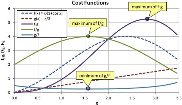
Note that points (2) and (3) appear to effectively describe the same scenario (we would only have to swap the functions); however, this is incorrect because the two functions are indeed dissimilar. We now want to plot these cases as shown in Figure 3-9. It can be seen that the maximum of f·g is near x = 2.8. For f/g it is near x = 1.6 and for g/f the maximums are near x = 0 and x = 3.5. The minimum is near x = 1.75.
EXAMPLE 3-2
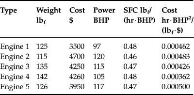
Five engine models are being considered for an airplane (see table below). It has been determined that all five will function well in the airplane, but we want to find out which engine is the best choice based on weight (W), cost (C), power (P), and fuel consumption (SFC) as listed below. Suggest cost functions that can be used to indicate the most suitable engine type.
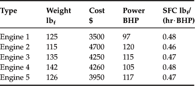
Solution
The approach is to maximize favorable properties and minimize unfavorable ones. For instance, we want the engine to have a low weight (W), be inexpensive (C), and have low fuel consumption (SFC). Assuming we put equal emphasis on all three, the engine with the lowest value of W × C × SFC is a potential winner. However, we also want the highest power possible. Therefore, an appropriate cost function would be:
![]()
This ratio is highest for an engine with high power, low weight, low price, and low SFC. It may not have the highest power or the lightest weight, but the most favorable combination of the selected characteristics. Calculated for the example engines, this would result in the following costs, which indicates Engine 5 is the best option:
Cost functions can be defined in other ways too. For instance, we could evaluate ratios such as power/weight (BHP/lbf), power/cost (BHP/$), and power/SFC (lbf·BHP²/hr). Since the high values of P/W, P/C, and P/SFC are desirable, a suitable cost function could be defined as the sum of these, i.e.
![]()
This would result in the following costs:

It can be seen that Engine 2 has the highest power-to-weight ratio, but the power-to-cost ratio of Engine 5 is the best. Overall, according to this scheme, Engine 2 is the best choice.
Sometimes it is desirable to emphasize one ratio above others. In other words, it is possible the power/weight ratio is of greater importance to the designer than, say, the power/cost ratio. This can be handled by introducing weighing fractions in a variety of ways. As an example, if the importance of P/W is considered 4 times more important than P/C and 10 times more important than P/SFC, we could introduce this as shown below:
![]()
Implementing these yields the following table:
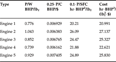
Again, for this example, Engine 2 comes out as the best option.
Exercises
(1) A single engine piston-engine propeller airplane is being designed to meet the following requirements:
(a) The design shall comply with LSA requirements as stipulated by ASTM F2245.
(b) Design gross weight shall be 1320 lbf in accordance with LSA requirements.
(c) It must sustain a 1.5g constant velocity turn while cruising at 100 KCAS.
(d) It must be capable of climbing at least 1000 fpm at 70 KCAS at S-L.
(e) It must be capable of operating from short runways in which the ground run is no greater than 500 ft and liftoff speed of 55 KCAS at design gross weight.
(f) It must be capable of a cruising speed of at least 110 KTAS at 8000 ft.
(g) It must be capable of a service ceiling of at least 14,000 ft.
The designer’s initial target is a minimum drag coefficient of 0.035 and an aspect ratio of 7. Furthermore, it is assumed the ground friction coefficient for the T-O requirement is 0.04, the T-O lift and drag coefficients are CL TO = 0.5 and CD TO = 0.04, respectively. Plot a constraint diagram for these requirements in terms of W/S and T/W for values of W/S ranging from 10 to 40 lbf/ft². Then, determine the required wing area and horsepower for the airplane if its propeller efficiency at cruise is 0.80, 0.7 during climb, and 0.6 at other low-speed operations.
(2) A twin piston-engine propeller airplane is being designed to meet the following requirements:
(a) Design gross weight shall be 5000 lbf.
(b) It must sustain a 1.5g constant velocity turn while cruising at 180 KTAS at 12,000 ft.
(c) It must be capable of climbing at least 1800 fpm at 100 KCAS at S-L.
(d) It must be capable of operating from short runways in which the ground run is no greater than 1200 ft and liftoff speed of 75 KCAS at design gross weight.
(e) It must be capable of a cruising speed of at least 180 KTAS at 12,000 ft.
(f) It must be capable of a service ceiling of at least 25,000 ft.
The designer’s initial target is a minimum drag coefficient of 0.035 and an aspect ratio of 7. Furthermore, it is assumed the ground friction coefficient for the T-O requirement is 0.04, the T-O lift and drag coefficients are CL TO = 0.5 and CD TO = 0.04, respectively. Plot a constraint diagram for these requirements in terms of W/S and T/W for values of W/S ranging from 10 to 40 lbf/ft². Then, determine the required wing area and horsepower for the airplane if its propeller efficiency at cruise is 0.80, 0.7 during climb, and 0.6 at other low speed operations.
(3) Prepare a stall speed–cruise speed carpet plot for a small twin-engine jet aircraft for which the following parameters are given:

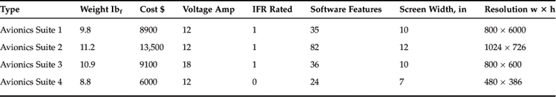
(4) Four avionics suites are being considered for a new small airplane (see table below) and you have been tasked with recommending one over the others. Using weight (W), cost (C), voltage (V), IFR rating (R), number of software features (F), screen width (S), and screen resolution area (w·h) as variables, suggest a cost function that can be used to indicate the most suitable avionics suite. (Hint: use the min or max of each column as a reference value, noting that low weight, cost, and voltage; IFR rating; high number of software features; large screen width and resolution are favorable).
Variables
| Symbol | Description | Units (UK and SI) |
| AR | Aspect ratio | |
| b | Wingspan | ft or m |
| bVT | Vertical tail span | ft or m |
| CD TO | Drag coefficient during T-O run | |
| CDmin | Minimum drag coefficient | |
| CL TO | Lift coefficient during T-O run | |
| CLmax | Maximum lift coefficient | |
| CLβVT | Vertical tail lift curve slope | per deg or per rad |
| CN | Yawing moment | lbf·ft or N·m |
| Cnβ | Directional stability derivative | deg−1 or rad−1 |
| DP | Propeller diameter | ft or m |
| e | Oswald efficiency | |
| g | Acceleration due to gravity | ft/s2 or m/s2 |
| H | Cruise altitude | ft or m |
| k | Coefficient for lift-induced drag | |
| KCAS | Knots calibrated airspeed | knots |
| KTAS | Knots true airspeed | knots |
| l0 | Basic length of a tail arm (to leading edge of tail root) | ft or m |
| lVT | Vertical tail moment arm | ft or m |
| LVT | Vertical tail lift force | lbf or N |
| n | Load factor | |
| P0 | Rated power (for propellers) | BHP |
| PBHP | Power of a piston engine | BHP |
| PS | Specific energy level | ft/s or m/s |
| q | Dynamic pressure | lbf/ft2 or N/m2 |
| qstall | Dynamic pressure @ stall condition | lbf/ft2 or N/m2 |
| ROC | Rate of climb | ft/min of m/min |
| S | Surface area | ft2 of m2 |
| SFC | Specific fuel consumption | lbf/(hr·BHP) |
| SG | Ground run | ft of m |
| SVT | Vertical tail surface area | ft2 or m2 |
| T | Thrust | lbf or N |
| T/W | Thrust-to-weight ratio | |
| T0 | Thrust at sea level | lbf or N |
| TREQ | Required thrust for specified condition | lbf or N |
| V | Airspeed | ft/s or m/s |
| VC | Cruise speed | ft/s or m/s |
| VLOF | Liftoff speed | ft/s or m/s |
| Vs | Stall speed | ft/s or m/s |
| VV | Vertical speed | ft/s m/s |
| W | Weight | lbf or N |
| W/S | Wing loading | lbf/ft2 or N/m2 |
| W0 | Gross weight | lbf or kg |
| μ | Ground friction constant | |
| η | Propeller efficiency factor | |
| λ | Taper ratio | |
| ΛVT | Vertical tail leading edge sweep | deg or rad |
| ρ | Density | slugs/ft3 or kg/m3 |
1For a list of packages see: http://en.wikipedia.org/wiki/List_of_statistical_packages.
2For a list of packages see: http://en.wikipedia.org/wiki/List_of_optimization_software.
3Per 14 CFR 23.49(d), Stalling period.
4Per 14 CFR 1.1, Definitions.