Chapter 1. First steps on the Cloud
In the previous two chapters, we frogmarched you through the essentials of genomics and computing technology. Our goal was to make sure you have enough of a grounding in both domains regardless of whether you’re coming to this more from one side or from the other — or perhaps even from another domain altogether; if so, welcome! And, hang on in there.
We realize that those first two chapters might have felt very passive since there were no hands-on exercises involved. So here’s the good news: you’re finally going to get to do some hands-on work! This chapter is all about getting you oriented and comfortable with the Google Cloud Platform (GCP) services that we’ll use throughout this book. First we’ll walk you through creating a GCP account and running some simple commands in Google Cloud Shell. After that, we’ll show you how to set up your own VM in the cloud, get Docker running on it and set up the environment that you’ll use in the next chapter to run GATK analyses. Finally, we’ll also show you how to configure the Integrative Genome Viewer (IGV) to access data in Google Cloud storage. Once you’ve got all that set up, you’ll be ready to do some actual genomics.
Setting up your Google Cloud account and first Project
You can sign up for an account on Google Cloud by navigating to https://cloud.google.com/ and following the prompts. If you don’t already have a Google identity of some kind, you can create one with your regular email account; you don’t have to use a Gmail account. Keep in mind also that if your institution uses G Suite, your work email may already be associated with a Google identity even if the domain name is not “gmail.com”.
Once you’ve signed up, make your way to the Google Cloud console, which provides a web-based graphical interface for managing cloud resources. Most of the functionality offered in the console can also be accessed through a pure command line interface. In the course of the book, we show you how to do some things through the web interface and some through the command line depending on what we believe is most convenient and/or typical.
Create a Project
Let’s start by creating your first Project, which is necessary to organize your work, set up billing and gain access to Google Cloud services. Go to the “Manage resources” page in the console at https://console.cloud.google.com/cloud-resource-manager and select “Create Project” at the top of the page. As shown in Figure 4-1, you’ll need to give your project a name, which must be unique within the entire Google Cloud Platform. You can also select an organization if your Google identity is associated with one (usually the case if you have an institutional/work G Suite account), but if you just created your account, this may not be applicable to you right now. Having an organization selected means new projects will be associated with that organization by default, which allows for central management of projects. For the purposes of these instructions we assume you’re setting up your account for the first time and there isn’t a pre-existing organization linked to it.
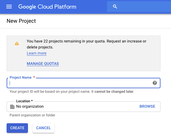
Figure 1-1. Creating a new project
Check your billing account and activate free credits
If you followed the signup process outlined above, the system will have set up billing information for you as part of the overall account creation process. You can check your billing information in the “Billing” section of the console at https://console.cloud.google.com/billing/, which you can also access at any time from the sidebar menu.
If you’re eligible for the free credits program, one of the panels on the billing overview page will summarize how many credits you have left and how many days you have left to spend them. Note that if yours is displaying a blue button labeled “Upgrade”, as shown in Figure 4-2, your trial has not yet started and you need to activate it in order to take advantage of the program. You may also see a “Free trial status” banner at the top of your browser window with a blue “Activate” button. Someone at Google Cloud is working really hard to not let you walk away from free money… So click either of those buttons to start the process and receive your free credits.
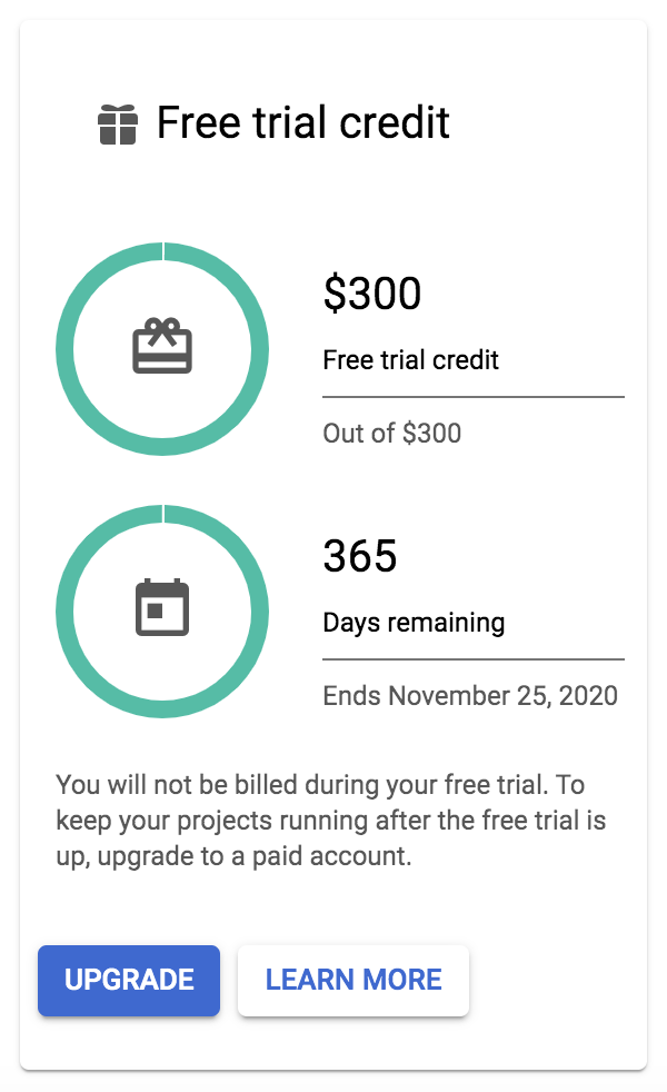
Figure 1-2. Panel in the Billing console summarizing free trial credits availability
More generally, the billing overview page provides summaries of how much money (or credits) you have spent so far, as well as some basic forecasting. That being said, it’s important to understand that the system does not show you costs in real time: there is some lag time between the moments when you use chargeable resources and when the costs get updated on your billing page.
Many people who make the move to cloud report that keeping track of their spending is one of the hardest parts of the process, and the one that causes them the most anxiety because it can be very easy to spend large sums of money pretty quickly on the cloud if you’re not careful. One feature offered by Google Cloud that we find particularly useful in this respect is the “Budgets & alerts” settings. This allows you to set email alerts that will notify you (or whoever is the billing administrator on your account) when you cross certain spending thresholds. To be clear, this won’t stop anything from running or prevent you from starting any new work that would take you over the threshold — but at least it will let you know where you stand.
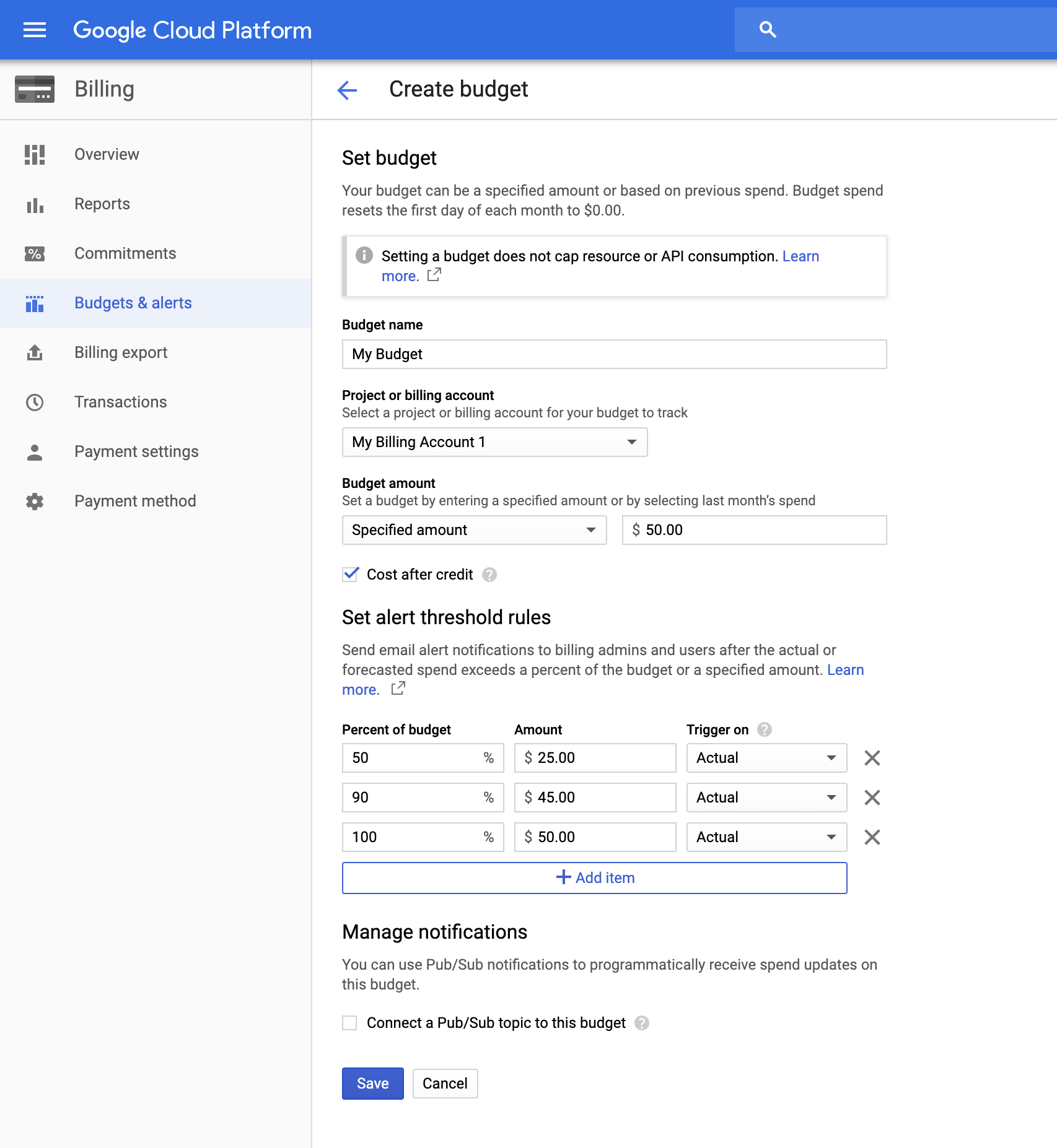
Figure 1-3. Budget and alert threshold administration
To access the billing notifications feature, choose “Billing” under the main menu on the Cloud Console, select the billing account you just created, and look for the “Budgets and alerts” option. Once you select it you will be able to setup a new budget using the “Create budget” form in Figure 4-3. You can create multiple budgets and set multiple triggers for different percentages of the budget if you want warnings as you get closer to your budget amount. But as we mentioned above, keep in mind that it is still only a notification service and will not prevent you from incurring additional charges.
Running basic commands in Google Cloud Shell
Now that you’ve established your account and set up billing the next step is to log into your first virtual machine (VM). We’ll use a service called Google Cloud Shell that does not require any configuration to get started and is completely free, although it comes with a few important limitations that we’ll discuss below.
Log into the Cloud Shell VM
To create a secure connection to a Cloud Shell VM using the Secure Shell (SSH) protocol, click on the terminal icon in the upper right hand corner of the console (Figure 4-4):

Figure 1-4. Terminal icon to open Cloud Shell
This launches a new panel in the bottom on the console; if you want you can also pop the terminal out into its own window. This gives you shell access to your own Debian-based Linux VM provisioned with modest resources, including 5GB worth of free storage (mounted at $HOME) on a persistent disk. Some basic packages are pre-installed and ready to go, including the Google Cloud SDK (a.k.a. gcloud), which provides a whole set of command line-based tools for interacting with Google Cloud services. We’ll use it in a few minutes to try out some basic data management commands. Feel free to explore this Debian VM now, look around, see what tools are installed.
Note
Be aware that there are weekly usage quotas that limit how much time you can spend running the Cloud Shell; currently 50 hours per week. In addition, if you don’t use it regularly (currently within 120 days), the contents of the disk that provides you with free storage may get deleted.
When you log into Cloud Shell for the first time, it will prompt you to specify a Project ID using the gcloud utility we just introduced above.
Welcome to Cloud Shell! Type "help" to get started.
To set your Cloud Platform project in this session use “gcloud config set project [PROJECT_ID]”
You can find your Project ID on the “Home” page of the console as shown in Figure 4-5.
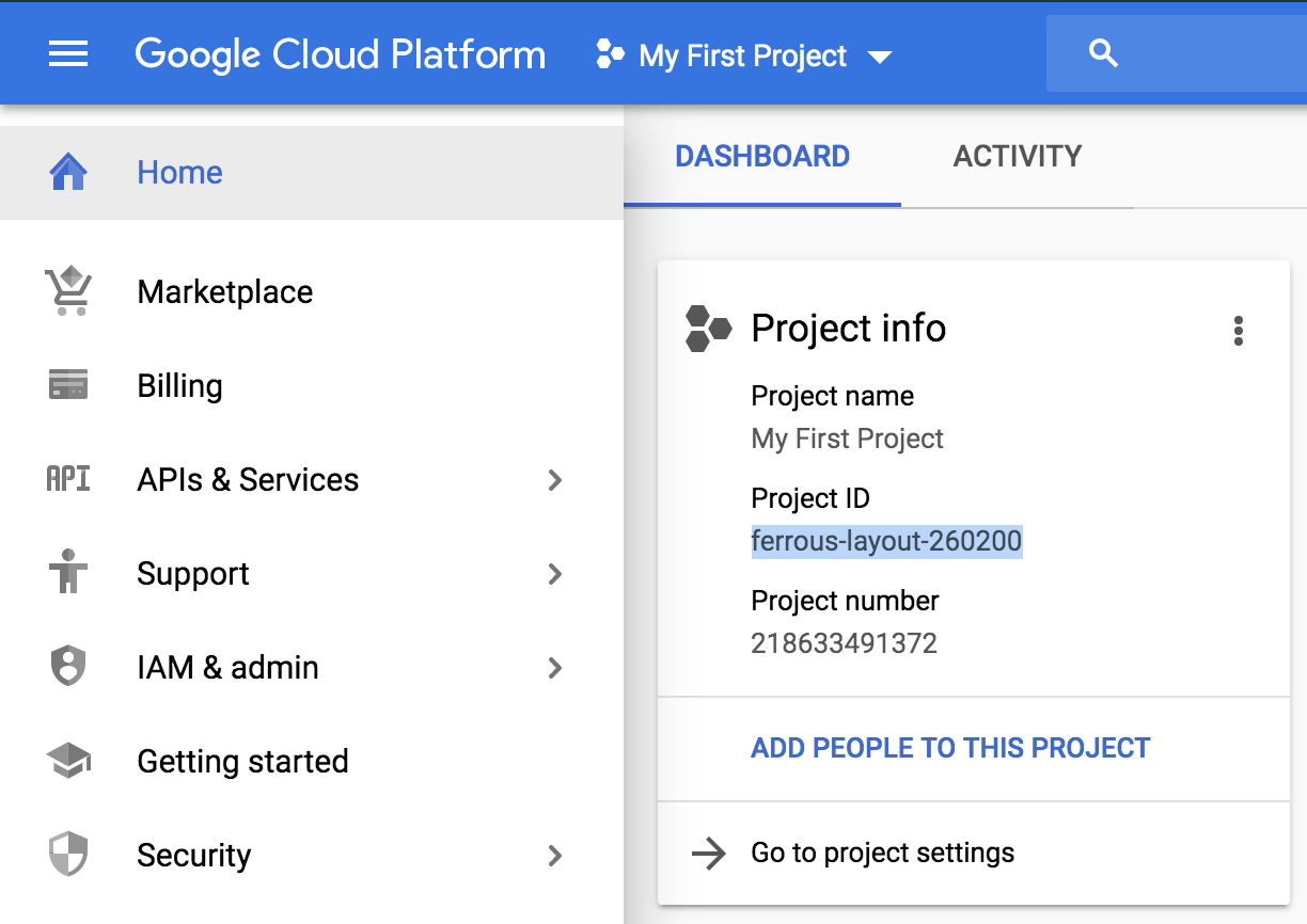
Figure 1-5. Location of the Project ID in the Google Cloud console.
Once you have your Project ID, run the following command in the Cloud Shell, substituting your own Project ID for the one shown below.
genomics_book@cloudshell:~$ gcloud config set project ferrous-layout-260200
Updated property [core/project].
genomics_book@cloudshell:~ (ferrous-layout-260200)$
Notice that your command prompt now includes your Project ID. That is all quite long so going forward, we’ll only show the last character in the prompt, in this case the dollar sign ($), when we demonstrate running commands. For example, if we list the contents of the working directory with the “ls” command, it’ll look like this:
$ ls
README-cloudshell.txt
And hey, there’s already something here: a README file, which as the name indicates really wants you to read it. You can do so by running the “cat” command:
$ cat README-cloudshell.txt
This will display a welcome message that summarizes some usage instructions and recommendations for getting help. And with that, you’re ready to use Cloud Shell to start interacting with basic Google Cloud services. Let’s get cracking!
Use gsutil to access and manage files
Now that we have access to this extremely simple-to-launch and free (if fairly limited VM) let’s use it to see if we can access the bundle of example data provided with this book. The data bundle lives in Google Cloud Storage (GCS), which is a form of “object store” (i.e. it’s used for storing files) with units of storage called “buckets”. You can view the contents of GCS buckets and perform some basic management tasks on them via the web through the storage browser section of the GCP console at https://console.cloud.google.com/storage/browser, but the interface is fairly limiting. The more powerful approach is to use the gcloud tool gsutil (which stands for Google Storage Utilities) from the command line. You can access buckets through their GCS path, which is just their name prefixed with “gs://”.
As an example, the path for the public storage bucket for this book is “gs://genomics-on-the-cloud”. You can list the contents of the bucket by typing the following command in your cloud shell:
$ gsutil ls gs://genomics-on-the-cloud
gs://genomics-on-the-cloud/hello.txt
gs://genomics-on-the-cloud/book-bundle-v0/
There should be a file called “hello.txt”. Let’s use the gsutil version of the Unix command “cat”, which allows us to read the content of text files, to see what this “hello.txt” file contains:
$ gsutil cat gs://genomics-on-the-cloud/hello.txt
HELLO, DEAR READER!
You can also try copying the file to your storage disk:
$ gsutil cp gs://genomics-on-the-cloud/hello.txt .
Copying gs://genomics-on-the-cloud/hello.txt...
/ [1 files][   20.0 B/   20.0 B]
Operation completed over 1 objects/20.0 B.
If you list the contents of your working directory with “ls” again, you should now have a local copy of the “hello.txt” file.
$ ls
hello.txt  README-cloudshell.txt
Since we’re playing with gsutil, how about we do something that will be useful later: let’s have you create a storage bucket of your own, so that you can store outputs in GCS. You’ll need to substitute “my-bucket” in the command shown below, as bucket names MUST be UNIQUE across all of GCS.
$ gsutil mb gs://my-bucket/
If you didn’t change the bucket name, or you tried a name that was already taken by someone else, you may get the following error message:
Creating gs://my-bucket/...
ServiceException: 409 Bucket my-bucket already exists.
If that’s your case, just try something else that’s more likely to be unique. You’ll know it worked when you only see the “Creating <name>...” in the output then get back to the prompt without any further complaint from gsutil.
Once that’s done, copy the “hello.txt” file to your new bucket. You can do either directly from the original bucket:
$ gsutil cp gs://genomics-on-the-cloud/hello.txt gs://my-bucket/
Or you can do it from your local copy, for example if you made modifications that you want to save:
$ gsutil cp hello.txt gs://my-bucket/
Finally, as one more example of basic file management, you can decide the file should live in its own directory in your bucket:
$ gsutil cp gs://my-bucket/hello.txt gs://my-bucket/my-directory/
As you can see, the gsutil commands are set up to be as similar as possible to their original Unix counterparts. So for example you’ll also be able to use “-r” to make the cp and mv commands recursive to apply to directories. For very large file transfers, there are a few cloud-specification optimizations that you can use to speed up the process, like the “gsutil -m” option which parallelizes file transfers. Conveniently, the system will usually tell you in the terminal output when you could take advantage of such optimizations, so you don’t need to go and memorize the documentation up front.
Pull a Docker image and spin up the container
Cloud Shell is the gift that keeps on giving: the Docker application (which we introduced in the previous chapter) comes pre-installed, so we can go ahead and get you started with that too! We’re going to use a simple Ubuntu container to illustrate basic Docker functionality. Although there is a Docker image available for GATK, and that’s what we’re going to use for a good chunk of the next few chapters, we’re not going to use it here because it’s rather large so it takes a little while to get going. We wouldn’t actually be able to run any realistic analyses with it in the free Cloud Shell because of the small amount of CPU and memory resources allocated for this free VM.
Note
The first thing to do to learn how to use Docker containers in this context is to.... avoid the online Docker documentation! Seriously. Not because it’s bad, but because the majority of those docs are written mainly for people who want to run web applications on the cloud. If that’s what you want to do, more power to you, but you’re reading the wrong book… What we’re providing here are tailored instructions that will teach you how to use Docker to run research software in containers.
As noted above, we’re going to use a very generic example: an image containing the Ubuntu Linux operating system. It’s an official image that is provided as part of the core library in the public container image repository Docker Hub, so we just need to state its name. You’ll see later that images contributed by the community are prefixed by the contributor’s username or organization name. Still in your Cloud Shell terminal (it doesn’t matter where your working directory is), run the following command to retrieve the Ubuntu image from the DockerHub library of official (certified) images:
$ docker pull ubuntu
Using default tag: latest latest: Pulling from library/ubuntu 7413c47ba209: Pull complete 0fe7e7cbb2e8: Pull complete 1d425c982345: Pull complete 344da5c95cec: Pull complete Digest: sha256:d91842ef309155b85a9e5c59566719308fab816b40d376809c39cf1cf4de3c6a Status: Downloaded newer image for ubuntu:latest docker.io/library/ubuntu:latest |
The pull command fetches the image and saves it to your VM. The version of the container image is indicated by its tag (which can be anything the image creator wants to assign) and by its sha256 hash (which is based on the image contents). By default the system gives us the latest version that is available because we did not specify a particular tag; in a later exercise we’ll see how to request a specific version by its tag. Note that container images are typically composed of several modular “slices”, which get pulled separately. They’re organized so that the next time you pull a version of the image, the system will skip downloading any slices that are unchanged compared to the version you already have.
Now let’s start up the container. There are three main options for running it, but the tricky thing is that there is usually only one right way to do it as its author intended and it’s hard to know what that is if the documentation doesn’t tell you (which is soooo often the case). Confused? Let’s walk through the case figures to make this a bit more concrete and you’ll see why we’re putting you through this momentary frustration and mystery -- it’s to save you potential misery down the road.
First option: just run it!
$ docker run ubuntu
Result: A short pause, then your command prompt comes back. No output. What happened? Docker did in fact spin up the container, but the container wasn’t configured to do anything under those conditions, so it basically shrugged and shut down again.
Second option: run it with a command appended.
$ docker run ubuntu echo "Hello World!"
Hello World!
Result: It echoed “Hello World!” as requested, then shut down again. Okay, so now we know that we can pass commands to the container, and if it’s a command that is recognized by something in there, it will be executed. Then when any and all commands have been completed, the container will shut down. A bit lazy, but reasonable.
Third option: run it interactively with the -it option.
$ docker run -it ubuntu /bin/bash
root@d84c079d0623:/#
Result: Aha, a new command prompt (bash in this case)! But with a different shell symbol, “#” instead of “$”. This means the container is running and we are in it. You can now run any command that you would normally use on an Ubuntu system, including installing new packages if you like. Try running a few Unix commands such as ls or ls -la to poke around and see what the container can do. Later in the book, particularly in Chapter 12, we’ll go into some of the implications of this, including some practical instructions for how to package and redistribute an image you’ve customized in order to share your own analysis in a reproducible way.
When you’re done poking around, type “exit” at the command prompt (or hit CTRL+d) to terminate the shell. Since this is the main process the container was running, terminating it will cause the container to shut down and return to the Cloud Shell itself. To be clear, this will shut down the container and any commands that are currently running.
If you’re curious, yes it is possible to step outside of the container without shutting it down; that’s called “detaching”. To do so, use CTRL+p+q instead of the exit command. You’ll then be able to jump back into the container at any time — provided you can identify it. By default, Docker assigns your container a universally unique identifier (UUID) as well as random human-readable name (which tend to sound a bit silly). You can run docker ps to list currently running containers or docker ps -a to list containers that have been created. This will display a list of containers indexed by their container IDs that should look something like this:
$ docker ps -a
CONTAINER ID        IMAGE               COMMAND                 CREATED              STATUS                          PORTS               NAMES
c2b4f8a0c7a6        ubuntu              "/bin/bash"             5 minutes ago   Up 5 minutes                       vigorous_rosalind
9336068da866        ubuntu              "echo 'Hello World!'"   8 minutes ago       Exited (0) 8 minutes ago                       objective_curie
We’re showing two entries correspond to the last two invocations of Docker, each with a unique identifier, the CONTAINER ID. We see the container with ID c2b4f8a0c7a6 that is currently running was named “vigorous_rosalind” and has a status of “Up 5 minutes”. You can tell that the other, “objective_curie”, is not running because its status is “Exited (0) 8 minutes ago”. The names we see here were randomly assigned (we swear! what are the odds) so they’re admittedly not terribly meaningful. If you have multiple containers running at the same time this can get a bit confusing, so you’ll want a better way to identify them. The good news is that you can give them a meaningful name by adding --name=meaningful_name right after docker run in your initial command, substituting meaningful_name with the name you want to give the container.
To enter the container, simply run docker attach c2b4f8a0c7a6, hit enter and you will find yourself back at the helm. You can open a second command tab in Cloud Shell if you’d like to be able to run commands outside the container alongside the work you’re doing inside the container. Note that you can have multiple containers running at the same time on a single VM — that’s one of the great advantages of the container system — but they will be competing for the CPU and memory resources of the VM, which in Cloud Shell are rather minimal. Later in this chapter we’ll show you how to spin up VMs with beefier capabilities.
Mounting a volume to access the filesystem from within the container
Having completed the previous exercise, you are now able to retrieve and run an instance of any container image shared in a public repository. There are many commonly used bioinformatics tools, including GATK, that are available pre-installed in docker containers. The idea is that knowing how to use them out of a docker means you won’t have to worry about having the right operating system or software environment. However, there’s still one trick we need to show you in order to make that really work for you: how to access your machine’s filesystem from within the container by “mounting a volume”.
What does that last bit mean? By default, when you’re inside the container you can’t access any data that lives on the filesystem outside of the container. The container is a closed box. There are ways to copy things back and forth between the container and your filesystem, but that gets tedious real fast. So we’re going to follow the easier path, which is to establish a link between a directory outside container in a way that makes it appear inside of the container. In other words, we’re going to poke a hole in the container wall, as shown in Figure 4-9.
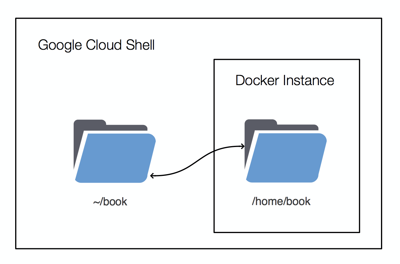
Figure 1-9. Mounting a volume or directory from your Google Cloud Shell into a Docker container.
As a toy example, let’s create a new directory called “book” in our Cloud Shell VM’s home directory, and put the “hello.txt” file from earlier inside of it.
$ mkdir book
$ mv hello.txt book/
$ ls book
hello.txt
So this time, let’s run the command to spin up our Ubuntu container with the -v argument (where v is for volume), which allows us to specify a filesystem location and a mount point within the container.
$ docker run -v ~/book:/home/book -it ubuntu /bin/bash
The -v ~/book_data:/home/book part of the command links the location you specified to the path /home/book inside the docker. The /home part of the path is a directory that already exists in the container, while the book part can be any name you choose to give it. Now, everything in the book directory on your filesystem can be accessed from within the docker container’s /home/book directory.
# ls home/book
hello.txt
Note
Here we’re using the same name for the mount point as for the actual location we’re mounting because it’s more intuitive that way, but you could use a different name if you wanted. Note that if you give your mount point the name of a directory or file that already exists with that path in the container, it will “squash” the existing path, meaning that path will not be accessible for as long as the volume is mounted.
There are a few other Docker tricks that are good to know, but for now, this is enough of a demonstration of the core Docker functionality that we’re going to use in the next chapter. We’ll go into the details of more sophisticated options as we encounter them.
Setting up your own custom VM
Now that you’ve successfully run some basic file management commands and got the hang of interacting with Docker containers, it’s time to move on to bigger and better things. The Google Cloud Shell environment is excellent for quickly getting started with some light coding and execution tasks but the VM allocated for Cloud Shell is really underpowered and will definitely not cut the mustard when it comes to running real GATK analyses in the next chapter.
In this section, we’re going to show you how to set up your own VM in the cloud (sometimes called “an instance”) using Google’s Compute Engine service, which allows you to select, configure and run VMs of whatever size you need.
Create and configure your VM instance
First, go to https://console.cloud.google.com/compute or access the page through the sidebar menu on the left as shown in Figure 10. When you click on the “VM Instances” link in this menu it will take you to an overview of running images. If this is a new account you won’t have any running. Notice at the top there’s an option for “Create Instance”. Click on that and we’ll walk through the process of creating a new VM with just the resources you need.

Figure 1-10. Compute Engine menu showing VM instances menu item
Next, in the top menu bar, click on “CREATE INSTANCE” as shown in Figure 4-11. This will bring up a configuration form as shown in Figure 4-12.

Figure 1-11. Create an instance
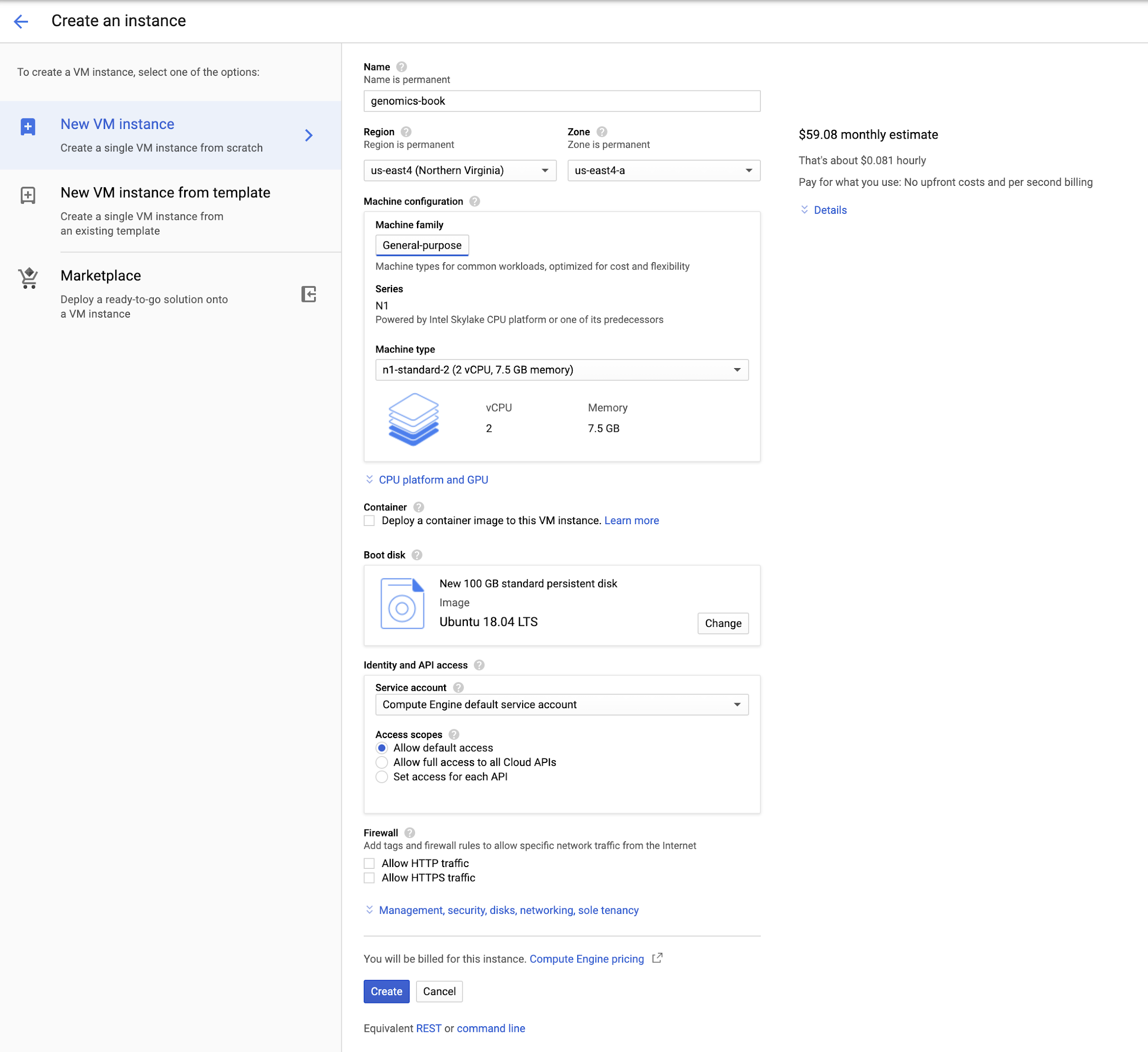
Figure 1-12. VM instance configuration panel
Follow the step by step instructions below to configure the VM. There are tons of options and it can be quite a confusing process if you don’t have experience with the terminology, so we mapped out the simplest path through the configuration form that will allow you to run all the command exercises in the first few chapters of this book. Please make sure you use exactly the same settings as shown here unless you really know what you’re doing.
Name your VM
Give your VM a name, for example “genomics-book”, as shown in Figure 4-13. This must be unique within your project but unlike bucket names, it does not need to be unique across GCP. Some people like to use their username so others with access to the project can instantly know who created the resource.
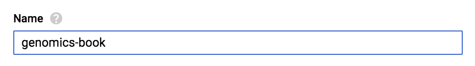
Figure 1-13. Name your VM instance
Choose a region (important!) and zone (not so important)
There are different physical locations for the cloud. Like most commercial cloud providers, Google Cloud maintains data centers in many different parts of the world and provides you with the option to choose which one you want to use. Regions are the top-level geographical distinction, with names that are reasonably descriptive like “us-west2” which refers to a facility in Los Angeles, California. Each region is further divided into two or more Zones designated by single letters (a, b, c etc), which correspond to separate data centers with their own physical infrastructure (power, network etc), though in some cases they might share the same building.
This system of regions and zones plays an important role in limiting the impact of localized problems like power outages, and all major cloud providers use some version of this strategy. For more on this topic, see this entertaining blog post by Kyle Galbraith about how cloud regions and zones (in his case, on AWS) could play an important role in the event of a zombie apocalypse.
Note
The ability to choose specific regions and zones for your projects is increasingly helpful for dealing with regulatory restrictions on where human subjects data can be stored since it allows you to specify a compliant location for all storage and compute resources. However, some parts of the world are not yet well covered by cloud services, or are covered differently by the various cloud providers, so you may need to factor in available data center locations when choosing a provider.
To choose a region for your project, you can consult the full list of available Google Cloud regions and zones and make a decision based on geographic proximity. Alternatively, you can use an online utility that measures how close you effectively are to each data center in terms of network response time, like http://www.gcping.com/. For example, if we run this test from the small town of Sunderland in Western Massachusetts (results in Table 1), we find that it takes 38 milliseconds to get a response from the us-east4 region located in Northern Virginia (698 km away), versus 41 milliseconds from the northamerica-northeast1 region located in Montreal (441 km away). This shows us geographical proximity does not correlate directly with network region proximity. As an even more striking example, we find that we are quite a bit “closer” to the europe-west2 region in London, UK (5,353 km away), with a response time of 102 milliseconds, than to the us-west2 region in Los Angeles, California (4,697 km away) which gives us a response time of 180 milliseconds.
| Region | Location | Distance (km) | Response (ms) |
| us-east4 | Northern Virginia, USA | 698 | 38 |
| northamerica-northeast1 | Montreal, Canada | 441 | 41 |
| europe-west2 | London, UK | 5,353 | 102 |
| us-west2 | Los Angeles, CA, USA | 4,697 | 180 |
Table 4-1: Geographical distance and response time from Sunderland, MA
Which brings us back to our VM configuration! For the Region, we’re going to be using us-east4 (Northern Virginia) since it’s closest to the one of us who travels least (GVdA), and for the Zone we just randomly choose us-east4-a. Please make sure you choose your region based on the discussion above, both for your own benefit (it’ll be faster) and to avoid clobbering that one data center in Virginia in the unlikely event that all 60,000 registered users of the GATK software start working through these exercises at the same time. Though that’s one way to test the vaunted elasticity of the cloud.
Select a machine type
This is the place where you can configure the resources of the VM you’re about to launch. You can control RAM as well as CPUs. For some instance types (available under Customize) you can even select VMs with Graphical Processing Units (GPUs), which are used to accelerate certain programs. The hitch is that what you select here will determine how much you’ll be billed per second of the VM’s uptime; the bigger and beefier the machine, the more it will cost you. The right side of the page should show how the hourly and monthly cost changes when you change the machine type. Note also that you’re billed for how long the VM is online, not for how much time you spend actually using it. We’ll cover strategies for limiting costs later, but keep that in mind!
Here we’re going to select “n1-standard-2”, a fairly basic machine that’s not going to cost us much at all, as shown in Figure 4-14.
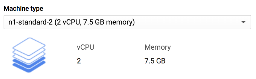
Figure 1-14. Select a machine type
Specify a container? (nope)
We’re not going to fill this out. This is useful if you want to use a very specific setup using a custom container image that you’ve preselected or generated yourself. In fact, we could have preconfigured a container for you and skipped a bunch of setup that’s coming next. But then you wouldn’t have the opportunity to learn how to do those things for yourself, would you… So for now, let’s just skip this option.
Customize the boot disk
Like Machine Type, this is another really useful setting. You can define two things here, the operating system you want to use and the amount of disk space you want. The former is especially important if you need to use particular type and version of operation system (OS). And of course the latter matters if you don’t want to run out of disk space halfway through your analysis.
By default the system proposes a particular flavor of Linux OS, accompanied by a paltry 10 GB of disk space, as shown in Figure 4-15. We’re going to need a bigger boat.
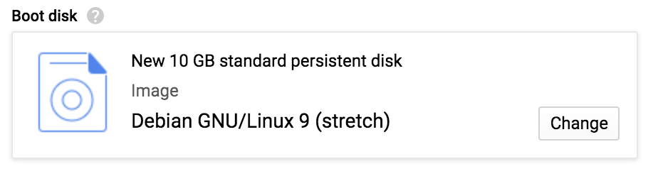
Figure 1-15. Choose a different boot disk
To access the settings menu for this, click “Change”. This opens a new screen with a fairly long list of predefined options. You can also make your own custom images, or even find more images in Google Cloud Marketplace (https://console.cloud.google.com/marketplace).
For our immediate purposes, we prefer Ubuntu 18.04 LTS, which is the most recent version of Ubuntu’s long term release at the time of this writing. It may not be as bleeding edge as Ubuntu 19.04 but the LTS, which stands for Long Term Support, guarantees that it’s being maintained for security vulnerabilities and package updates for 5 years from release. This Ubuntu image has a ton of what we already need ready to go and installed, including various standard Linux tools and the Google Cloud SDK command line tools which we will rely on quite heavily.
Select the Ubuntu 18.04 LTS image by clicking the radio button as shown in Figure 4-16.
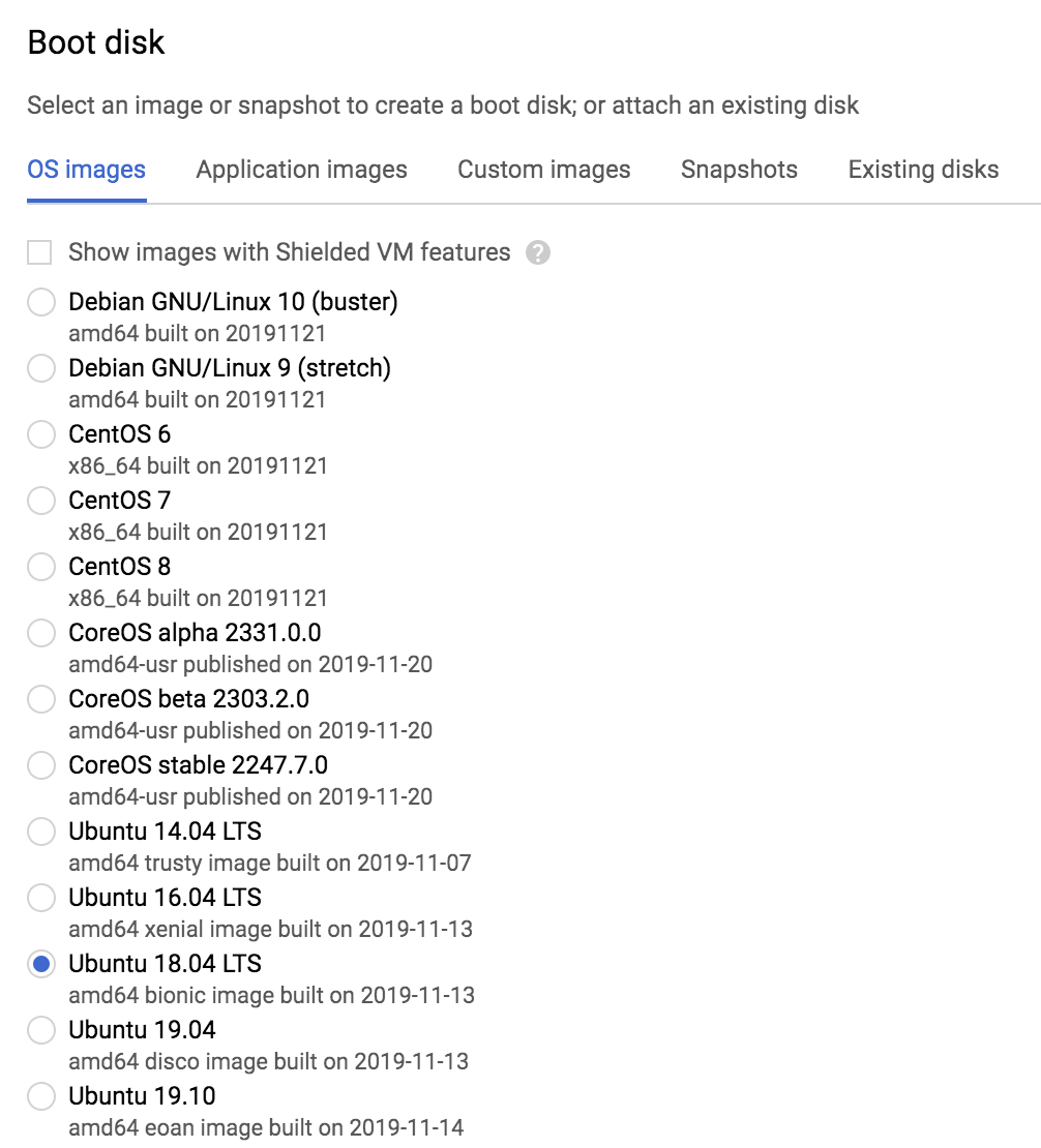
Figure 1-16. Select a base image
At the bottom of the form, you can change the Boot disk Size to give yourself more space. As shown in Figure 4-17, let’s select 100 GB instead of the default 10GB, since the data we’re going to be working with can easily take up a lot of space. You can bump this up quite a bit more depending on your dataset size and needs. While it can’t easily be adjusted after the VM launches, you do have the option of adding additional block storage volumes to the running instance after launch — think of it as the cloud equivalent of plugging in a USB drive. So if you run out of disk space you won’t be totally stuck.
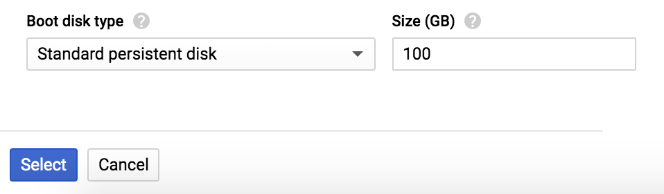
Figure 1-17. Set the boot disk size
Once you’ve done all this, click “Select”; this closes the screen and returns you to the instance creation form, where the “Boot disk” section should match the screenshot in Figure 4-18.
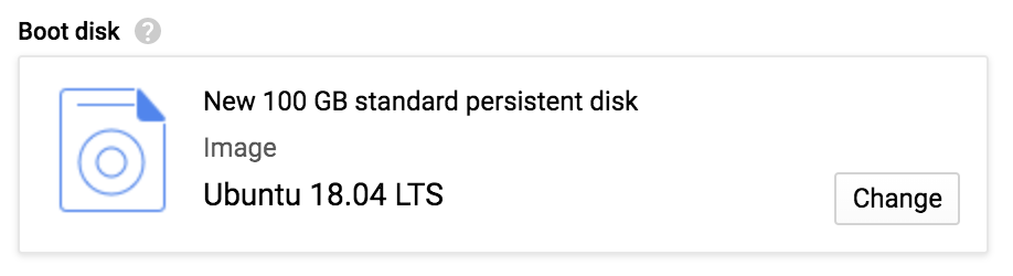
Figure 1-18. Updated boot disk selection
Click “Create” at the bottom of the form. This returns you to the page that lists Compute Engine VM instances, including your newly created VM instance. You may see a spinning icon in front of its name while the instance is being created and booted up, then a green circle with a check mark will appear when it is running and ready for use, as shown in Figure 4-19.
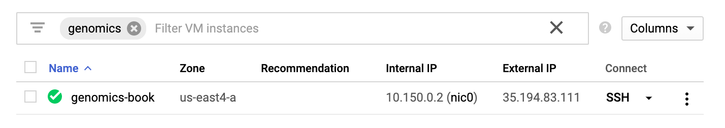
Figure 1-19. View VM status.
And voilà, your VM is ready for action.
Log into your VM with SSH
There are several ways that you can access the VM once it’s running, which you can learn about from the Google Cloud documentation. We’re going to show you the simplest way to do it, using the Google Cloud Console and the built-in SSH terminal. It’s hard to beat: once you see a green check mark in the Google Cloud Console, you can simply click on the SSH option as shown in Figure 4-20. Select the option “Open in a browser window” and a few seconds later you should see an SSH terminal open to this VM.
Note
Alright we’ll show you one other one, if you insist. Here it is: you can also use the gcloud command line to SSH to your VMs. The syntax is the following:
gcloud compute ssh --project [PROJECT_ID] --zone [ZONE] [INSTANCE_NAME]
You would need to replace the [PROJECT_ID], [ZONE] and [INSTANCE_NAME] with actual values (but no brackets). You can do this from the Cloud Shell VM or from any other location where you have installed the Google Cloud SDK command line package (gcloud). When you run it for the first time, the system may prompt you to generate an authentication key. Just follow the fairly straightforward prompts: type Y for yes then type your desired passphrase if you want to use one.

Figure 1-20. Options for SSHing into your VM
Once your VM status indicates that it’s ready, click on “SSH” (under the “Connect” column header) as instructed above. This will open a new window with a terminal that allows you to run commands from within the VM instance, as shown in Figure 4-21. It may take a minute to establish the connection.
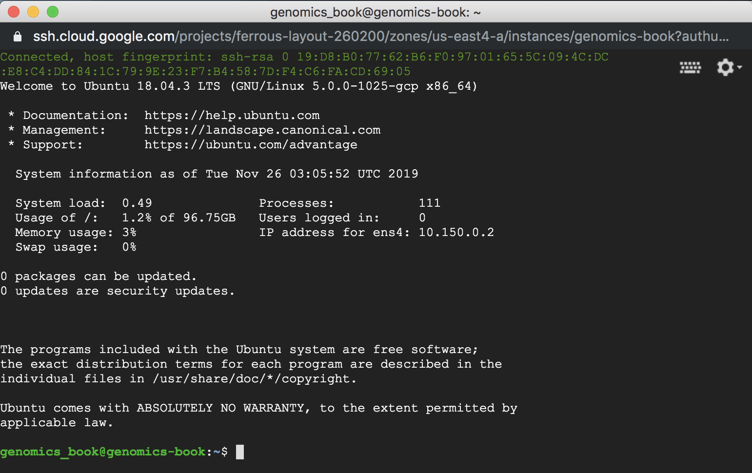
Figure 1-21. VM instance terminal
Feel free to look around and get to know your brand new VM; you’re going to spend a lot of time with it in the course of the next few chapters (but, like, in a good way).
Check your authentication
You’re probably itching to run something interesting, but let’s start by making sure your account credentials are set up properly so you can use the Google Cloud command line tools, which come preinstalled on the image we chose. Run the following command in the SSH terminal:
$ gcloud init
Welcome! This command will take you through the configuration of gcloud.
Your current configuration has been set to: [default]
You can skip diagnostics next time by using the following flag:
 gcloud init --skip-diagnostics
Network diagnostic detects and fixes local network connection issues.
Checking network connection...done.
Reachability Check passed.
Network diagnostic passed (1/1 checks passed).
Choose the account you would like to use to perform operations for
this configuration:
[1] [email protected]
[2] Log in with a new account
Please enter your numeric choice:
The line that starts with [1] shows you that by default Google Cloud has you logged in under a service account: the domain is @developer.gserviceaccount.com. This is fine for running tools within your VM, but if you want to be able to manage resources from inside there, including copying files out to GCS buckets, you need to do so under an account with the relevant permissions. It is possible to grant this service account all the various permissions that you’ll need for these exercises, but that would lead us a bit further into the guts of Google Cloud account administration than we’d like to go right now — we want to get you doing genomics work ASAP! So instead, let’s just use the original account that you used to create the project at the beginning of this chapter since it already has those permissions as a project owner.
To log in with that account, type “2” at the prompt. This will trigger some interaction with the program; Google Cloud will warn you that using your personal credentials on a VM is a security risk because if you give someone else access to the VM, they will be able to use your credentials. The solution: don’t share access to your personal VM1.
You are running on a Google Compute Engine virtual machine.
It is recommended that you use service accounts for authentication.
You can run:
 $ gcloud config set account `ACCOUNT`
to switch accounts if necessary.
Your credentials may be visible to others with access to this
virtual machine. Are you sure you want to authenticate with
your personal account?
Do you want to continue (Y/n)?
If you type “Y” for Yes, the program will give you a link.
Go to the following link in your browser:
   https://accounts.google.com/o/oauth2/auth?redirect_uri=<...>
Enter verification code:
When you click the link or copy and paste it into your browser, you will be presented with a Google login page. Log in to get your authentication code, then copy and paste that back into your terminal window. The gcloud utility will confirm your login identity and ask you to select the project ID you want to use from the list of projects you have access to. It will also offer the option to set your preferred compute and storage zone, which should match what you set earlier when you created the VM. If you’re not seeing what you expect in the project ID list, you can always double-check the resource management page in the Google Cloud console at https://console.cloud.google.com/cloud-resource-manager.
Copy the book materials to your VM
Throughout the next few chapters, you’re going to run real GATK commands and workflows on your VM, so you need to retrieve the example data, source code and a couple of software packages. To make it easy, we’ve bundled all of that in a single place: a Google Cloud Storage bucket called genomics-on-the-cloud. You’re going to copy all of it over to your VM in a dedicated directory using gsutil, the Google Cloud storage utility that we already used earlier in the Cloud Shell portion of this chapter.
Note
We are committed to providing long term support and maintenance for the book contents, so we are making the source code available in a public repository on GitHub, a highly popular platform for sharing code under version control. If you’re not familiar with GitHub, don’t worry — we’ll walk you through the key points in Chapter 12, when we cover tools and approaches for sharing your own work in a reproducible manner.
In your VM’s terminal window, make a new directory called “book”:
$ mkdir book
Now, run the following command to copy the book data bundle to the storage space associated with your VM using gsutil:
$ gsutil -m cp -r gs://genomics-on-the-cloud/book-bundle-v0/* book/
This will copy about 10 Gb of data to your VM’s storage, so it may take a few minutes. As we’ll see later, it is possible to run some analysis commands directly on files in Google Cloud Storage without copying them first, but we want to keep things as simple as possible for now.
Install Docker on your VM
Now let’s make sure you can run Docker on your VM. If you simply run the command “docker” in the terminal, you’ll get an error message because Docker does not come preinstalled on the VM.
$ docker
Command 'docker' not found, but can be installed with:
snap install docker     # version 18.09.9, or
apt  install docker.io
See 'snap info docker' for additional versions.
The error message helpfully points out how to remedy the situation using a pre-installed package called snap, but we’re actually going to use a slightly different way of installing Docker: we’re going to download and run a script from the Docker website that will largely automate the installation process. This way, you’ll know what to do if you find yourself in the situation of needing to install Docker somewhere that doesn’t have a built-in package manager option.
Run the following command to install Docker on the VM:
$ curl -sSL https://get.docker.com/ | sh
# Executing docker install script, commit: f45d7c11389849ff46a6b4d94e0dd1ffebca32c1
+ sudo -E sh -c apt-get update -qq >/dev/null
...
Client: Docker Engine - Community
Version:           19.03.5
...
If you would like to use Docker as a non-root user, you should now consider
adding your user to the "docker" group with something like:
 sudo usermod -aG docker genomics_book
Remember that you will have to log out and back in for this to take effect!
WARNING: Adding a user to the "docker" group will grant the ability to run
        containers which can be used to obtain root privileges on the
        docker host.
        Refer to https://docs.docker.com/engine/security/security/#docker-daemon-attack-surface
        for more information.
This may take a little while to complete so let’s take that time to examine the command in a bit more detail. First, we’re using a convenient little utility called curl (short for “Client URL”) to download the installation script from the Docker website URL we provided, with a few command parameters (-sSL) that tell the program to follow any redirection links and save the output as a file. Then we use the pipe character (|) to hand that output file over to a second command, sh, which means “run that script that we just gave you”. The first line of output tells you what it’s doing: “Executing docker install script” (we omitted parts of the output above for brevity).
When it finishes, the script will prompt you to run the usermod command below in order to grant yourself the ability to run Docker commands without using “sudo” each time. Invoking “sudo docker” can result in output files being owned by root, making it difficult to manage or access them later, so it’s really important to do this step.
$ sudo usermod -aG docker $USER
This does not produce any output; we’ll test in a minute whether it worked properly. First however you need to log out of your VM and then back in again. Doing so will make the system re-evaluate your Unix group membership, which is necessary for the change you just made to take effect. Simply type “exit” (or hit CTRL+d) at the command prompt:
$ exit
This closes the terminal window to your VM. Go back to the Google Cloud Console, find your VM in the list of Compute Engine instances and click “SSH” to log back in again. This probably feels like a lot of hoops to jump through, but hang on in there, we’re getting to the good part.
Set up the GATK container image
Once you’re back in your VM, test your Docker installation by pulling the GATK container, which we’ll use in the very next chapter:
$ docker pull broadinstitute/gatk:4.1.3.0
4.1.3.0: Pulling from broadinstitute/gatk
ae79f2514705: Pull complete
5ad56d5fc149: Pull complete
170e558760e8: Pull complete
395460e233f5: Pull complete
6f01dc62e444: Pull complete
b48fdadebab0: Pull complete
16fb14f5f7c9: Pull complete
Digest: sha256:e37193b61536cf21a2e1bcbdb71eac3d50dcb4917f4d7362b09f8d07e7c2ae50
Status: Downloaded newer image for broadinstitute/gatk:4.1.3.0
docker.io/broadinstitute/gatk:4.1.3.0
As a reminder, the last bit after the container name is the version tag, which you can change to get a different version than what we’ve specified here. Note that if you change the version, there may be some commands that no longer work. We can’t guarantee that all code examples are going to be future-compatible, especially for the newer tools, some of which are still under active development. See the book’s GitHub repository for updated materials, as noted earlier.
The GATK container image is quite large so the download may take a little while. The good news is that next time you need to pull a GATK image (e.g. to get another release), Docker will only pull the components that have been updated, so it will go faster.
Now, remember the instructions you followed earlier in this chapter to spin up a container with a mounted folder? You’re going to use that again to make the book directory accessible to the GATK container.
$ docker run -v ~/book:/home/book -it broadinstitute/gatk:4.1.3.0 /bin/bash
You should now be able to browse the book directory that you set up in your VM from within the container. It will be located under “/home/book”. Finally, to double-check that GATK itself is working as expected, try running the command “gatk” at the command line from within your running container. If everything is working properly, you should see some text output that outlines basic GATK command line syntax and a few configuration options.
# gatk
Usage template for all tools (uses --spark-runner LOCAL when used with a Spark tool)
   gatk AnyTool toolArgs
Usage template for Spark tools (will NOT work on non-Spark tools)
   gatk SparkTool toolArgs  [ -- --spark-runner <LOCAL | SPARK | GCS> sparkArgs ]
Getting help
   gatk --list       Print the list of available tools
   gatk Tool --help  Print help on a particular tool
Configuration File Specification
    --gatk-config-file                PATH/TO/GATK/PROPERTIES/FILE
gatk forwards commands to GATK and adds some sugar for submitting spark jobs
  --spark-runner <target>    controls how spark tools are run
    valid targets are:
    LOCAL:      run using the in-memory spark runner
    SPARK:      run using spark-submit on an existing cluster
                --spark-master must be specified
                --spark-submit-command may be specified to control the Spark submit command
                arguments to spark-submit may optionally be specified after --
    GCS:        run using Google cloud dataproc
                commands after the -- will be passed to dataproc
                --cluster <your-cluster> must be specified after the --
                spark properties and some common spark-submit parameters will be translated
                to dataproc equivalents
  --dry-run      may be specified to output the generated command line without running it
  --java-options 'OPTION1[ OPTION2=Y ... ]'   optional - pass the given string of options to t
he
                java JVM at runtime.
                Java options MUST be passed inside a single string with space-separated values
.
We’ll discuss what that all means in loving detail in the next chapter; for now you’re done setting up the environment that you’ll be using to run GATK tools over the course of the next three chapters.
Stop your VM… to stop it from costing you money
The VM you just finished setting up is going to come in handy throughout the book; we’ll have you come back to this VM for many of the exercises in the next few chapters. However, as long as it’s up and running, it’s costing you either credits or actual money. The simplest way to deal with that is to stop it, i.e. put it on pause whenever you’re not actively using it. You’ll be able to restart it on demand; it just takes a minute or two to get it back up and running, and it will retain all environment settings, the history of what you ran previously and whatever data you have in local storage. Note that you will be charged a small fee for that storage even while the VM is not running and you’re not getting charged for the VM itself. In our opinion, this is well worth it for the convenience of being able to come back to your VM after some arbitrary amount of time and just pick up your work where you left off.
To stop your VM, go to the VM instances management page in the Google Cloud console as shown previously. Find your instance and click on the three-dot symbol on the right to pull up the menu of controls, then select “Stop” as shown in Figure 4-22. It may take a couple of minutes for the process to complete, but you can safely navigate away from that page. To restart your instance later on, just follow the same steps but click on “Start” in the control menu.
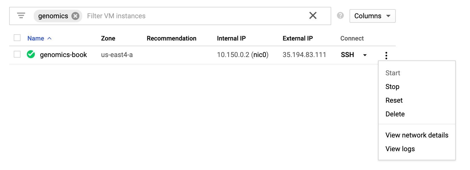
Figure 1-22. Stopping, starting or deleting your VM instance.
Alternatively, you can delete your VM entirely, but keep in mind that deleting the VM will delete all locally stored data too, so make sure you save anything you care about to a storage bucket first.
Configure the Integrated Genome Viewer to read data from GCS buckets
There’s just one more small step to go before you move on to the next chapter: we’re going to install and configure a genome browser called Integrated Genome Viewer (IGV) that can work directly with files in Google Cloud. That will allow you to examine sequence data and variant calls without needing to copy the files to your local machine.
First, if you don’t have it installed yet on your local machine, get the IGV program from the website at https://software.broadinstitute.org/software/igv/download and follow the installation instructions. If you already have a copy, consider updating it to the latest version; we are using 2.6.2. Open the application; click on the “View” menu item in the top menu bar and select “Preferences” in the dropdown menu that is displayed as shown in Figure 4-23.

Figure 1-23. Location of the “Preferences” menu item.
This opens the Preferences pane, shown below in Figure 4-24.
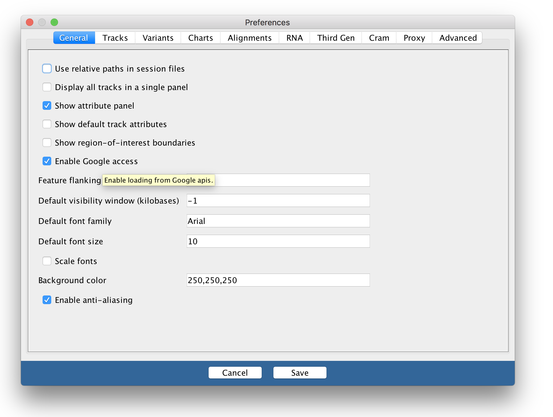
Figure 1-24. IGV “Preferences” pane
In the Preferences pane, check the box titled “Enable Google access” and click Save, then quit IGV and reopen it to force a refresh of the top menu bar. You should now see a “Google” menu item that was not there previously. Click on it and select “Login …” as shown in Figure 4-25 to set up IGV with your Google account credentials.
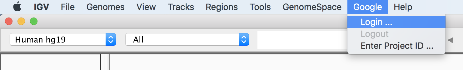
Figure 1-25. Google “Login ...” menu item
This will take you to a Google login page in your web browser; follow the prompts to allow IGV to access relevant permissions on your Google account. Once this is complete, you should see a webpage that simply says “OK”. Let’s switch back to IGV and test that it works. In the top-level menu, click on “Files” and select “Load from URL...” as shown in Figure 4-26, making sure not to select one of the other options by mistake. They look similar so it’s easy to get tripped up. Make sure also that the reference dropdown menu in the top left corner of the IGV window is set to “Human hg19”. If you’re confused about what is different between the human references, see the notes in Chapter 2 about Hg19 and GRCh38.
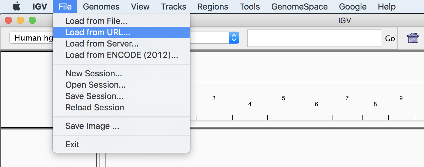
Figure 1-26. “Load from URL” menu item
Finally, enter the GCS file path for one of the sample BAM files we provide in the book data bundle in the dialog window that pops up (for example, the mother.bam as shown in Figure 4-27), then click OK. Remember, you can get a list of files in the bucket by using gsutil from your VM or from Cloud Shell, or you can browse the contents of the bucket by using the Google Cloud console storage browser. If you use the browser interface to get the path to the file, you’ll need to compose the GCS file path by stripping off the first part of the URL before the bucket name, i.e. remove "https://console.cloud.google.com/storage/browser/" and replace that by “gs://”. Do the same for the BAM’s accompanying index file which should have the same file name and path but end in “.bai”.
For example, "https://console.cloud.google.com/storage/browsergenomics-on-the-cloud/book-bundle-v0/data/germline/bams/mother.bam" becomes “gs://genomics-on-the-cloud/book-bundle-v0/data/germline/bams/mother.bam”.
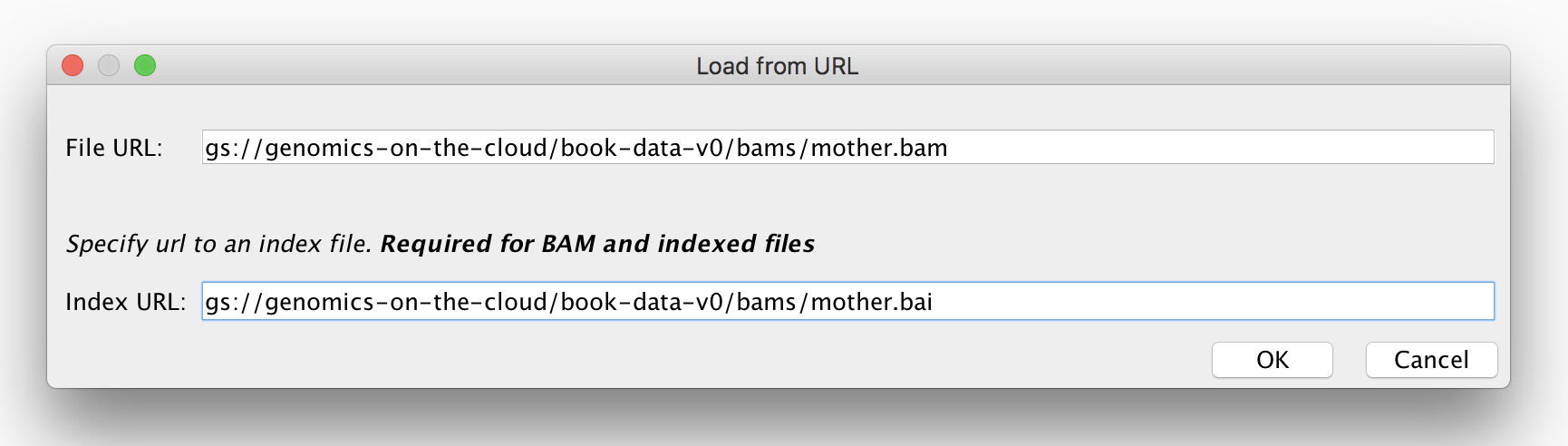
Figure 1-27. “Load from URL” dialog
This will make the data available to you in IGV as a new data track, but by default nothing will be loaded in the main viewer. To check that you can view data, enter the genomic coordinates 20:9,999,830-10,000,170 in the search window and click Go. These coordinates will take you to the 10 millionth DNA base +/- 170 on the 20th human chromosome, as shown in Figure 4-28, where you’ll see the left-side edge of the slice of sequence data that we provide in this sample file. We’ll explain in detail how to interpret the visual output of IGV in the next chapter, when we use it to investigate the result of a real (small) analysis.
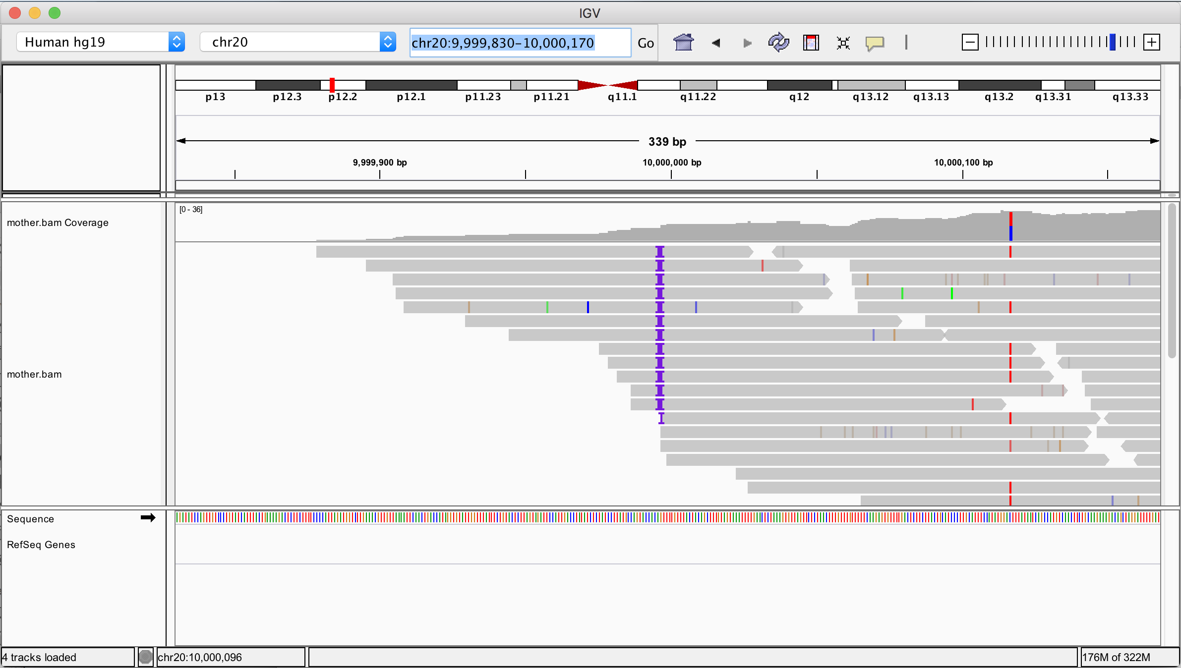
Figure 1-28. IGV view of BAM file located in a GCS bucket
IGV only retrieves small slices of data at a time, so the transfer should be very fast unless you have a particularly slow internet connection. Do keep in mind however that Google Cloud, like all commercial cloud providers, will charge an egress fee for transferring data out of the cloud. On the bright side, it’s a very small fee, proportional to the amount of data you transfer. So the cost of viewing slices of data in IGV is trivial — on the order of fractions of pennies — and it is definitely preferable to what it would cost to transfer the entire file for offline browsing!
You can view the contents of other data files, like VCFs, using the same set of operations, as long as the files are stored in a Google Cloud bucket. Unfortunately that means this won’t work for files that are on the local storage of your VM, so anytime you want to examine one of those, you’ll need to copy it to a bucket first. You’re going to get real friendly with gsutil in no time...
Oh, one last thing while you’ve got IGV open: click the little yellow callout bubble in the IGV window toolbar, which controls the behavior of the detail viewer, as shown in Figure 4-29. Do yourself a favor and switch the setting from “Show Details on Hover” to “Show Details on Click”. Whichever action you choose will trigger the appearance of little dialog that gives you detailed information about any part of the data that you either click or hover over; for example for a sequence read, it will give you all the mapping information as well as the full sequence and base qualities. You can try it out now with the data you just loaded. As you’ll see, the detail display functionality in itself is very convenient, but the “on hover” version of this behavior can be a bit overwhelming when you’re new to the interface, hence our recommendation to switch to “on click”.
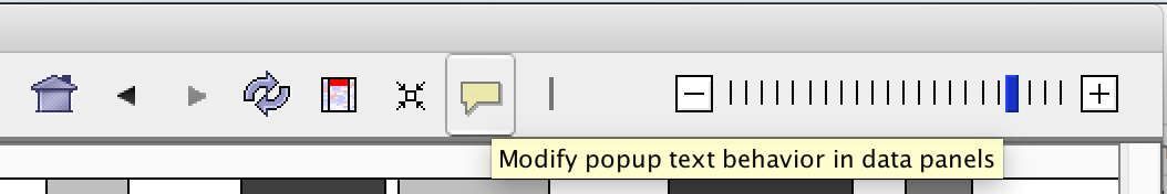
Figure 1-29. Change the behavior of the detail viewer from “on Hover” to “on Click”
Wrap up and next steps
In this chapter, we showed you how to get started with Google Cloud resources, from creating an account, using the super-basic Google Cloud Shell, then graduating to your own custom Virtual Machine. You learned how to manage files in Google Cloud Storage, run Docker containers and administer your VM. Finally, you retrieved the book data and source code, finished setting up your custom VM to work with the GATK container and set up IGV to view data stored in buckets. In the next chapter, we’ll get you started with GATK itself, and before you know it you’ll be running real genomics tools on example data in the cloud.
1 Keep in mind that if you create accounts for other users in your Google Cloud project, they will be able to SSH to your VMs as well. It is possible to further restrict access to your VMs in a shared project but that is beyond the simple introduction we’re presenting here.