Operating requirements

Because GATK is written in Java, you can run it almost anywhere as long as you have the right version of Java installed on your machine (at time of writing, JRE or JDK 1.8), except on Microsoft Windows, which is not supported. There is no installation necessary in the traditional sense; in its simplest form, all you need to do is download the GATK package, place its contents in a convenient directory on your hard drive (or server filesystem) and, optionally, add the location of the gatk wrapper script to your PATH.

However, a subset of tools (especially the newer ones that use fancy machine learning libraries) have additional R and/or Python dependencies, which can be quite painful to install. Also, this exposes you to annoying conflicts with the requirements of other tools that you may need to use. For example, let’s say you are using a version of GATK that requires numpy==1.13.3 but you also need to use a different tool that requires numpy==1.12.0. This could quickly become a nightmare, where you update a package to enable one analysis only to find later that another of your scripts no longer runs successfully.

You can use a package manager like Conda to mitigate this problem. There is an official GATK Conda script that you can use to replicate the environment required for GATK, but frankly, it’s not a perfect solution.

The best way to deal with this is to use a container, which provides a fully self-contained environment that encapsulates all requirements and dependencies, as described in Chapters 3 (theory) and 4 (practice). Every GATK release comes with a container image that matches that version’s requirements exactly, and it’s just a “docker pull” away. That means no more time and effort wasted setting up and managing your work environment, a huge win for portability and reproducibility of complex analyses.

Multithreading with Spark

Earlier versions of the GATK used some home-grown, hand-rolled code to provide multithreading functionality. If you’re an old-timer you may be familiar with the GATK engine arguments -nt and -nct. Starting with GATK4 all that is gone; the GATK team chose to replace it with Spark, which has emerged as a much more robust, reliable and performant option. The relevant Spark library is bundled inside GATK itself, so there is no additional software to install. It works right out of the box, on just about any system — contrary to surprisingly widespread belief, you do not need a special Spark cluster to run Spark-enabled tools. However, some tools have computational requirements that exceed the capabilities of single-core machines. As we’ll see at several points in this book, one of the advantages of cloud infrastructure is that we’re able to pick and choose suitable machines on demand depending on the needs of a given analysis.

To use Spark multithreading, the basic syntax is fairly straightforward: we just need to add a few arguments to the regular GATK command line. Note that when we add Spark arguments, we first add a -- separator that consists of two dashes, which tells the parser system that what follows is intended for the Spark subsystem.

In the simplest case, called “local execution”, the program executes all the work on the same machine where we’re launching the command. To do that, simply add --spark-master local[*] to the base command line. The --spark-master local part tells the Spark subsystem to send all work to the machine’s own local cores, and the value in brackets specifies the number of cores to use. To use all available cores, replace the number by an

$ gatk MySparkTool 
	-R data/reference.fasta 
	-I data/sample1.bam 
	-O data/variants.vcf 
	-- 
	--spark-master local[4]

If you have access to a Spark cluster, the Spark-enabled tools are going to be extra happy, though you may need to provide some additional parameters to use them effectively. We don’t cover that in detail here, but here are examples of the syntax you would use to send the work to your cluster depending on your cluster type:

• Run on the cluster at 23.195.26.187, port 7077
  --spark-master spark://23.195.26.187:7077
  

• Run on the cluster called my_cluster in Google Dataproc
  --spark-runner GCS --cluster my_cluster

That covers just about all you need to know about Spark for now, because using the cloud allows us to sidestep some of the issues that made Spark so valuable in other settings. However, it will pop up again in Chapter 11, when we show you how to scale up and speed up interactive analyses in the cloud.

Running GATK in practice

By this point you’re probably itching to run some actual GATK commands, so let’s get started. We’re going to assume you are using the virtual machine that we had you set up in Chapter 4, and that you have also already pulled and tested the GATK container image as instructed in that same chapter.

If your VM is still up and running, go ahead and SSH back into it, unless you never even left. If it’s stopped, head on over to the Google Cloud console VM instance management page, start your VM and log back into it.

$ docker run -v ~/book:/home/book -it broadinstitute/gatk:4.1.3.0 /bin/bash

(gatk) root@ce442edab970:/gatk# 

# ls
GATKConfig.EXAMPLE.properties   gatk-package-4.1.3.0-spark.jar  gatkenv.rc
README.md                       gatk-spark.jar                  install_R_packages.R
book-data                       gatk.jar                        run_unit_tests.sh
gatk                            gatkPythonPackageArchive.zip    scripts
gatk-completion.sh              gatkcondaenv.yml
gatk-package-4.1.3.0-local.jar  gatkdoc

# gatk
Usage template for all tools (uses --spark-runner LOCAL when used with a Spark tool)
   gatk AnyTool toolArgs
Usage template for Spark tools (will NOT work on non-Spark tools)
   gatk SparkTool toolArgs  [ -- --spark-runner <LOCAL | SPARK | GCS> sparkArgs ]
Getting help
   gatk --list       Print the list of available tools
   gatk Tool --help  Print help on a particular tool
Configuration File Specification
    --gatk-config-file                PATH/TO/GATK/PROPERTIES/FILE
gatk forwards commands to GATK and adds some sugar for submitting spark jobs
  --spark-runner <target>    controls how spark tools are run
    valid targets are:
    LOCAL:      run using the in-memory spark runner
    SPARK:      run using spark-submit on an existing cluster
                --spark-master must be specified
                --spark-submit-command may be specified to control the Spark submit command
                arguments to spark-submit may optionally be specified after --
    GCS:        run using Google cloud dataproc
                commands after the -- will be passed to dataproc
                --cluster <your-cluster> must be specified after the --
                spark properties and some common spark-submit parameters will be translated
                to dataproc equivalents
  --dry-run      may be specified to output the generated command line without running it
  --java-options 'OPTION1[ OPTION2=Y ... ]'   optional - pass the given string of options to t
he
                java JVM at runtime. 
                Java options MUST be passed inside a single string with space-separated values
.

# gatk HaplotypeCaller --help

# cd /home/book/data/germline
# mkdir sandbox

# gatk HaplotypeCaller 
	-R ref/ref.fasta 
	-I bams/mother.bam 
	-O sandbox/mother_variants.vcf 

Using GATK jar /gatk/gatk-package-4.1.3.0-local.jar
Running:
   java -Dsamjdk.use_async_io_read_samtools=false -Dsamjdk.use_async_io_write_samtools=true -Dsamjdk.use_async_io_wri
te_tribble=false -Dsamjdk.compression_level=2 -jar /gatk/gatk-package-4.1.3.0-local.jar HaplotypeCaller -R ref/ref.fas
ta -I bams/mother.bam -O sandbox/mother_variants.vcf
09:47:17.371 INFO  NativeLibraryLoader - Loading libgkl_compression.so from jar:file:/gatk/gatk-package-4.1.3.0-local.
jar!/com/intel/gkl/native/libgkl_compression.so
09:47:17.719 INFO  HaplotypeCaller - ------------------------------------------------------------
09:47:17.721 INFO  HaplotypeCaller - The Genome Analysis Toolkit (GATK) v4.1.3.0
09:47:17.721 INFO  HaplotypeCaller - For support and documentation go to https://software.broadinstitute.org/gatk/
09:47:17.722 INFO  HaplotypeCaller - Executing as root@3f30387dc651 on Linux v5.0.0-1011-gcp amd64
09:47:17.723 INFO  HaplotypeCaller - Java runtime: OpenJDK 64-Bit Server VM v1.8.0_191-8u191-b12-0ubuntu0.16.04.1-b12
09:47:17.724 INFO  HaplotypeCaller - Start Date/Time: August 20, 2019 9:47:17 AM UTC

09:47:18.347 INFO  ProgressMeter - Starting traversal
09:47:18.348 INFO  ProgressMeter -        Current Locus  Elapsed Minutes     Regions Processed   Regions/Minute
09:47:22.483 WARN  InbreedingCoeff - InbreedingCoeff will not be calculated; at least 10 samples must have called geno
types
09:47:28.371 INFO  ProgressMeter -          20:10028825              0.2                 33520         200658.5
09:47:38.417 INFO  ProgressMeter -          20:10124905              0.3                 34020         101709.1
09:47:48.556 INFO  ProgressMeter -          20:15857445              0.5                 53290         105846.1
09:47:58.718 INFO  ProgressMeter -          20:16035369              0.7                 54230          80599.5
09:48:08.718 INFO  ProgressMeter -          20:21474713              0.8                 72480          86337.1
09:48:18.718 INFO  ProgressMeter -          20:55416713              1.0                185620         184482.4

09:48:20.714 INFO  ProgressMeter - Traversal complete. Processed 210982 total regions in 1.0 minutes.
09:48:20.738 INFO  VectorLoglessPairHMM - Time spent in setup for JNI call : 0.045453468000000004
09:48:20.739 INFO  PairHMM - Total compute time in PairHMM computeLogLikelihoods() : 6.333675601
09:48:20.739 INFO  SmithWatermanAligner - Total compute time in java Smith-Waterman : 6.18 sec
09:48:20.739 INFO  HaplotypeCaller - Shutting down engine
[August 20, 2019 9:48:20 AM UTC] org.broadinstitute.hellbender.tools.walkers.haplotypecaller.HaplotypeCaller done. Ela
psed time: 1.06 minutes.
Runtime.totalMemory()=717225984

# gatk ValidateSamFile 
    -R ref/ref.fasta 
    -I bams/mother.bam 
    -O sandbox/mother_validation.txt

HaplotypeCaller in a nutshell

HaplotypeCaller is designed to identify germline SNPs and indels with a high level of sensitivity and accuracy. One of its distinguishing features is that it uses local de-novo assembly of haplotypes to model possible variation. If that sounds like word salad to you, all you really need to know is that whenever the program encounters a region showing signs of variation, it completely realigns the reads in that region before proceeding to call variants. This allows the HaplotypeCaller to gain accuracy in regions that are traditionally difficult to call, for example when they contain different types of variants close to each other. It also makes the HaplotypeCaller much better at calling indels than traditional position-based callers like the old UnifiedGenotyper and Samtools mpileup.

HaplotypeCaller operates in four distinct stages illustrated in Figure 5-3 and outlined below. Note that this description refers to established computational biology terms and algorithms that we chose not to explain in detail here; if you would like to learn more about these concepts, we recommend asking the GATK support team for pointers to appropriate study materials.

1. Define active regions. The tool determines which regions of the genome it needs to operate on, based on the presence of significant evidence for variation, such as mismatches or gaps in read alignments.

2. Determine haplotypes by re-assembly of the active region. For each active region, the program builds a De Bruijn-like assembly graph to realign the reads within the bounds of the active region. This allows it to make a list of all the possible haplotypes supported by the data. The program then realigns each haplotype against the reference sequence using the Smith-Waterman algorithm in order to identify potentially variant sites.

3. Determine likelihoods of the haplotypes given the read data. For each active region, the program then performs a pairwise alignment of each read against each haplotype using the PairHMM algorithm. This produces a matrix of likelihoods of haplotypes given the read data. These likelihoods are then marginalized to obtain the likelihoods of alleles per read for each potentially variant site.

4. Assign sample genotypes. For each potentially variant site, the program applies Bayes’ rule, using the likelihoods of alleles given the read data to calculate the posterior probabilities of each genotype per sample given the read data observed for that sample. The most likely genotype is then assigned to the sample.

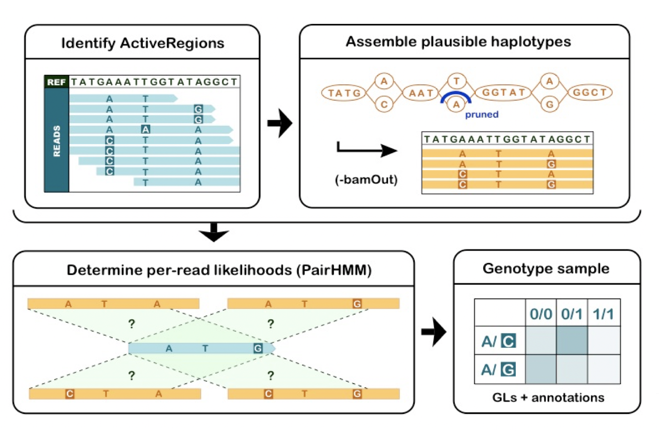
Figure 2-3. The 4 stages of HaplotypeCaller’s operation

The final output of HaplotypeCaller is a VCF file containing variant call records, which include detailed genotype information and a variety of statistics that describe the context of the variant and reflect the quality of the data used to make the call.

Run HaplotypeCaller and examine output

Let’s run HaplotypeCaller in its simplest form on a single sample to get familiar with its operation. This command requires a reference genome file in FASTA format (-R), as well as one or more files with the sequence data to analyze in BAM format (-I). It will output a file of variant calls in VCF format (-O). Optionally the tool can take an interval or list of intervals to process (-L), which we use here to restrict analysis to a small slice of data in the interest of time. This can also be used for the purpose of parallelizing execution, as we’ll see a little later in this book.

# gatk HaplotypeCaller 
	-R ref/ref.fasta 
	-I bams/mother.bam 
	-O sandbox/mother_variants.200k.vcf 
	-L 20:10,000,000-10,200,000

Once the command has run to completion (after about a minute), we need to copy the output file to a bucket so that we can view it in IGV, as we demonstrated at the end of Chapter 4. The simplest way to do this is to open a second SSH terminal to the VM from the Google console so that we can run gsutil commands, which is more convenient to do from outside the container. If at any point you lose track of which window is which, or where you should be running a given command, remember that the VM prompt ends in a dollar sign ($) and the container prompt ends in a hash (#). Just match them up and you’ll be okay.

Note

Alternatively, you can also copy the files directly from within the container, but first you have to run gcloud init as described in Chapter 4 from within the container, which has its own authentication scope.

In the second SSH terminal window that is now connected to your VM, move from the home directory into the germline sandbox directory.

$ cd ~/book/data/germline/sandbox

Next, you’re going to want to copy the contents of the sandbox directory to the storage bucket you created in Chapter 4 using the gsutil tool. However, it’s going to be annoying if you have to constantly replace the name we use for our bucket with your own, so let’s take a minute to set up on environment variable. It’s going to serve as an alias, so that you can just copy-paste our commands directly from now on.

Create the BUCKET variable by running the following command, replacing the “my-bucket” bit with the name of your own bucket as you did in Chapter 4 (last time!).

$ export BUCKET="gs://my-bucket"

Now check that the variable was set properly by running echo, making sure to add the dollar sign in front of BUCKET:

$ echo $BUCKET
gs://my-bucket

Finally, you can copy the file you want to view to your bucket.

$ gsutil cp mother_variants.200k.vcf* $BUCKET/germline-sandbox/
Copying file://mother_variants.200k.vcf [Content-Type=text/vcard]...
Copying file://mother_variants.200k.vcf.idx [Content-Type=application/octet-stream]...
- [2 files][101.1 KiB/101.1 KiB]                                               
Operation completed over 2 objects/101.1 KiB.

Once the copy operation is complete, you’re going to go to your desktop IGV application and load the reference genome, the input BAM file and the output VCF file. We covered that procedure in Chapter 4, so you may feel comfortable doing that on your own. But just in case it’s been a while, let’s go through the main steps together briefly. Feel free to refer to the screenshots in Chapter 4 if you need a refresher.

All of the actions in the numbered list below are to be performed in the IGV application unless otherwise specified.

1. In IGV, check in the top menu that your Google login is active.

2. Check that you have the “Human hg19” reference selected in the pulldown menu on the left. Technically our data is aligned to b37, but for pure viewing purposes (NOT analysis), the two are interchangeable.

3. Go to the File menu in the top menu bar, select “Load from URL” and paste the file path for the BAM file into the top field. You can leave the second field blank if you’re using IGV version 2.6.2 or later; IGV will automatically retrieve the index file. Click OK.

4. gs://genomics-on-the-cloud/book-bundle-v0/data/germline/bams/mother.bam

5. Get the file path for the output VCF file that you just copied to your bucket. You can get it by running “echo $BUCKET/germline-sandbox/” in your VM terminal.

6. Go to the File menu in the top menu bar, select “Load from URL” and paste the VCF file path that you got from the previous step in the first field. You can leave the second field blank again. Click OK.

At this point you should have all the data loaded and ready to go, but you don’t see anything yet because by default IGC shows you the full span of the genome, and at that scale the small slice of data we’re working with is not visible. To zoom in on the data, enter the coordinates 20:10,002,294-10,002,623 in the location box and click Go. You should see something very similar to Figure 5-4.

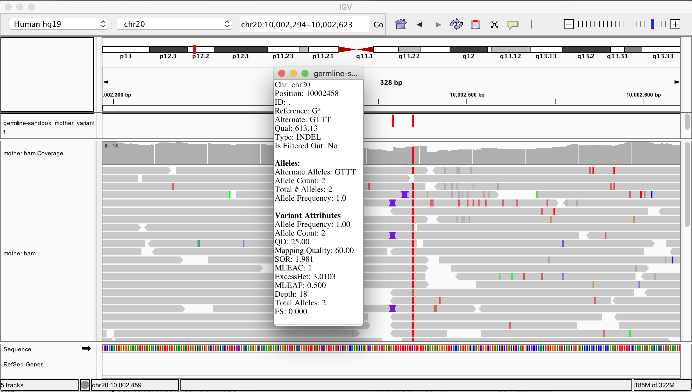
Figure 2-4. Original BAM file and output VCF file loaded in IGV.

The variant track showing the contents of the VCF file is displayed on top, and below is the read data track showing the contents of the BAM file. Variants are indicated as small vertical bars (colored in red in Figure 4) and sequence reads are represented as grey bars with a pointy bit indicating the read orientation. In the read data, we see various mismatches (small colored bars) and gaps (purple symbols for insertions; deletions would show up as black horizontal bars).

We see that HaplotypeCaller called two variants within this region. You can click on each little red bar in the variant track to get more details on each one. On the right, we have a homozygous SNP with excellent support in the read data. That seems very likely to be correct. On the left, we have a homozygous insertion of three T bases, yet we only see a very small proportion of reads with the purple symbol that support this call. How is this possible, when so few reads seem to support an insertion at this position?

Your first reflex when you encounter something like this (a call that doesn’t make sense, especially if it’s an indel) should be to turn on the display of soft-clipped sequence in the genome viewer you’re using. “Soft clips” are segments of reads that are marked by the mapper (in this case BWA) as being not useful, so they are hidden by default by IGV. The mapper introduces soft clips in the CIGAR string of a read when it encounters bases, typically toward the end of the read, that it is not able to align to the reference to its satisfaction based on the scoring model it employs. At some point the mapper gives up trying to align the bases, and just puts in the “S” operator to signify that downstream tools should disregard the following bases, even though they are still present in the read record. Some mappers even remove those bases, which is called hard clipping and uses the “H” operator instead of “S”.

Soft clips are interesting to us because they often occur in the vicinity of insertions, especially large insertions. So let’s turn on soft clips in IGV in the Preference; go to the View menu in the top menu bar, select Preferences and click on the Alignments tab to bring up the relevant settings. Find the checkbox labeled “Show soft-clipped bases” and check it as shown in Figure 5-5, then click Save to close the Preferences pane.

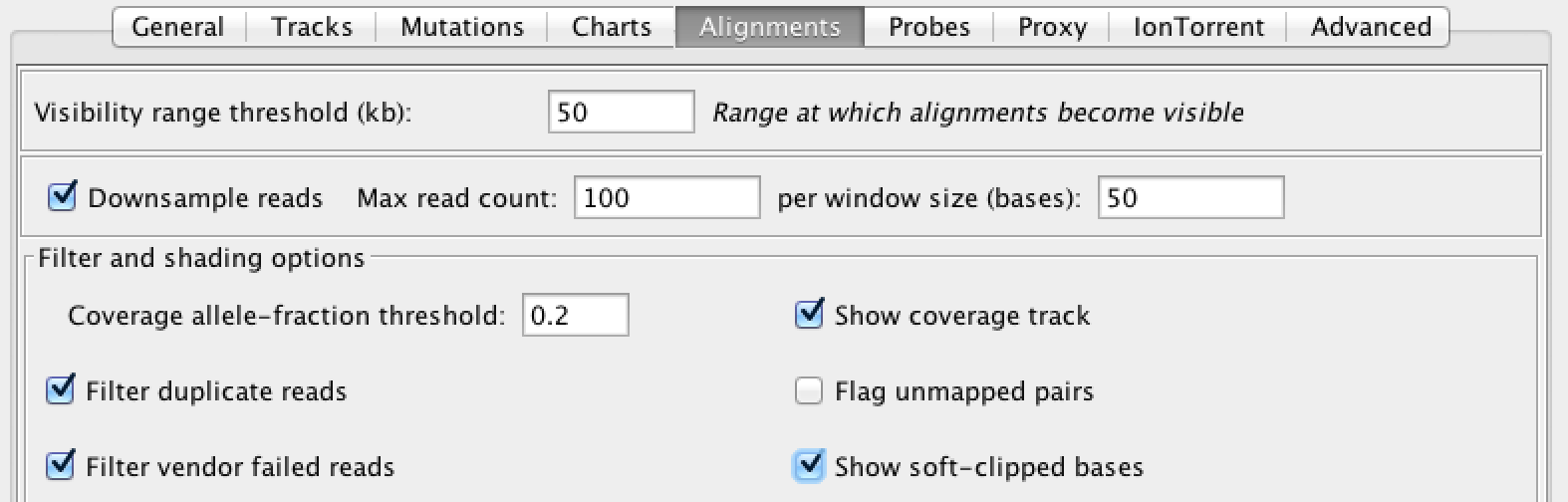
Figure 2-5. IGV alignment settings.

As we see in Figure 5-6, with soft clip display turned on, the region we’ve been looking at lights up with mismatching bases! That’s a fair amount of sequence that we were just ignoring because BWA didn’t know what to do with it. HaplotypeCaller, on the other hand, will have taken it into account when it called variants, since the first thing it does within an active region is to throw out all the read alignment information and build a graph to realign them, as we discussed earlier.

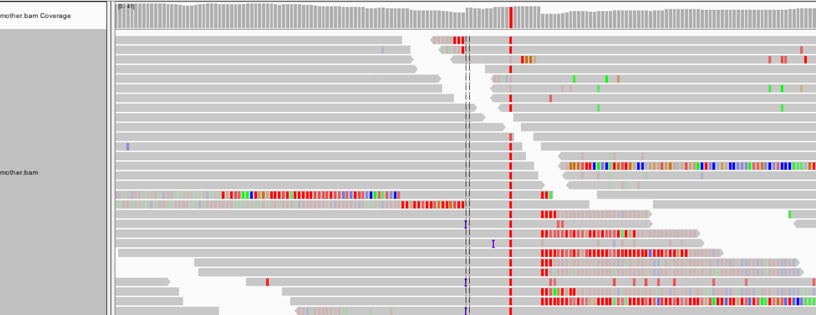
Figure 2-6. Turning on the display of soft clips shows a lot of information that was hidden.

So now we know that HaplotypeCaller had access to this additional information, and somehow decided that it supported the presence of an insertion at this position. But the extra sequence we see here is unaligned, so how can we check HaplotypeCaller’s work? Well, the tool has a parameter called -bamout, which makes HaplotypeCaller output a BAM file showing the result of the assembly graph-based realignment it performs internally. That’s great because it means we can see exactly what HaplotypeCaller saw when it made that call.

Generate an output BAM to troubleshoot a surprising call

Let’s generate the bamout so we can get a better understanding of what HaplotypeCaller thinks it’s seeing here. Run the following command, which should look very similar: it’s basically the same as the previous one except we changed the name of the output VCF (to avoid overwriting the first one), we narrowed the interval we’re looking at, and we specified a name for the realigned output BAM file using the new -bamout argument. As a reminder, we’re running this from the /home/book/data/germline directory.

# gatk HaplotypeCaller 
    -R ref/ref.fasta 
    -I bams/mother.bam 
    -O sandbox/mother_variants.snippet.debug.vcf 
    -bamout sandbox/mother_variants.snippet.debug.bam 
    -L 20:10,002,000-10,003,000

Since we’re only interested in looking at that particular region, we give the tool a narrowed interval with -L 20:10,002,000-10,003,000, to make the runtime shorter.

Once that has run successfully, copy the output BAM to your bucket then load it in IGV as we’ve previously described. It should load in a new track at the bottom of the viewer, as shown in Figure 5-7. You should still be zoomed in on the same coordinates (20:10,002,294-10,002,623), and have the original mother.bam track loaded for comparison. If you have a small screen, you can switch the view setting for the BAM files to “Collapsed” by right-clicking anywhere in the window where you see sequence reads.

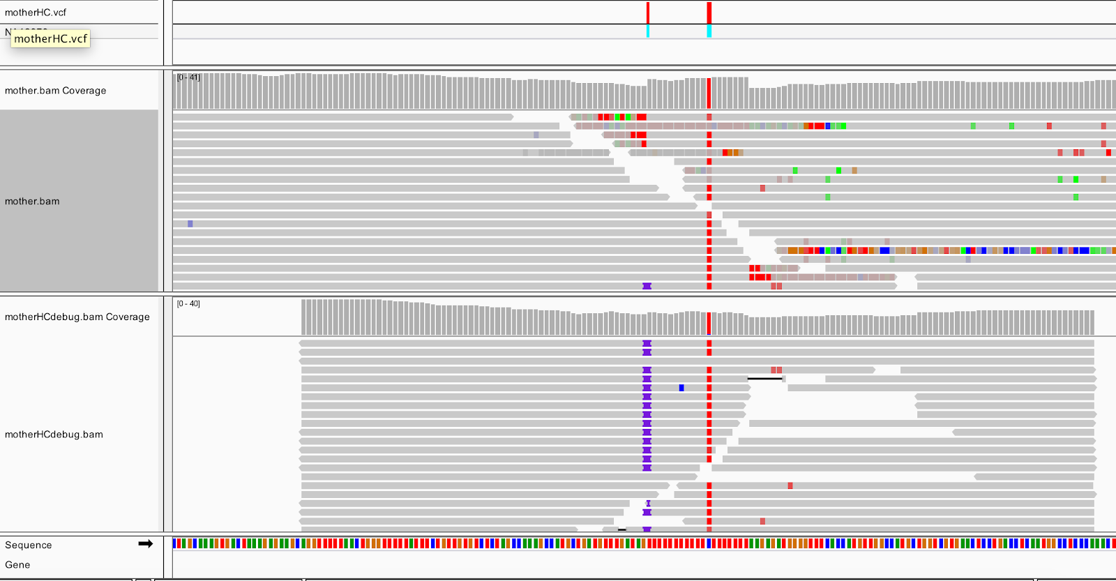
Figure 2-7. Realigned reads in the bamout file (bottom track).

The bottom track shows us that after realignment by HaplotypeCaller, almost all the reads support the insertion, and the messy soft clips that we see in the original BAM file are gone. This confirms that HaplotypeCaller utilized the soft-clipped sequences during the realignment stage and took that sequence into account when calling variants. Incidentally, if you expand the reads in the output BAM (right-click>Expanded view), and you can see that all of the insertions are in phase with the neighboring C/T variant. Such consistency tends to be a good sign; whereas if you had inconsistent segregation between neighboring variants, you would worry that at least one of them is an artifact.

So to summarize, this shows that HaplotypeCaller found a different alignment after performing its local graph assembly step. The reassembled region provided HaplotypeCaller with enough evidence to call the indel, whereas a position-based caller like UnifiedGenotyper would have missed it.

That being said, there is still a bit more to the bamout than meets the eye — or at least, what you can see in this view of IGV. Right-click on the mother_variants.snippet.debug.bam track to bring up the view options menu. Select Color alignments by, and choose read group. Your gray reads should now be colored similar to the screenshot below (Figure 5-8).

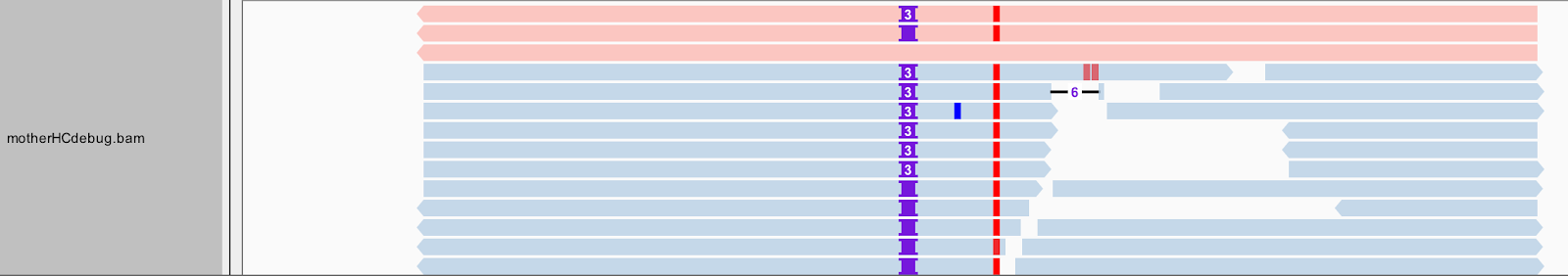
Figure 2-8. Bamout shows artificial haplotypes constructed by HaplotypeCaller.

Some of the first reads, those shown in red at the top of the pile in Figure 5-8, are not real reads. These represent artificial haplotypes that were constructed by HaplotypeCaller, and are tagged with a special read group identifier, RG:Z:ArtificialHaplotypeRG to differentiate them from actual reads. You can click on an artificial read to see this tag under Read Group.

Interestingly, the tool seems to have considered three possible haplotypes, including two with insertions of different lengths: either two bases or three bases inserted, before ultimately choosing the three-base case as being most likely to be real. To examine this a bit more closely, let’s separate these artificial reads to the top of the track. Right-click on the track to select “Group alignments by” and choose “read group”. Next let’s color the reads differently. Right-click and select “Color alignments by”, choose tag, and type in “HC”. HaplotypeCaller labels reads that have unequivocal support for a particular haplotype with an HC tag value that refers to the corresponding haplotype. So now the color shows us which reads in the lower track support which of the artificial haplotypes in the top track, as we can see in Figure 5-9. Gray reads are unassigned, which means there was some ambiguity about which haplotype they support best.

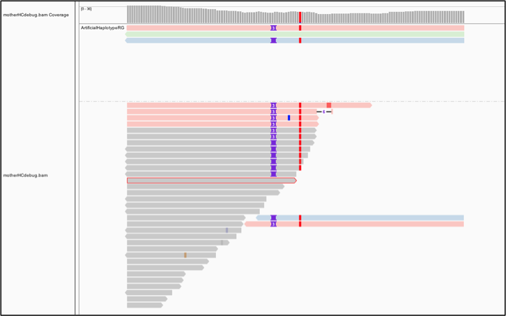
Figure 2-9. Bamout shows support per-haplotype.

This shows us that HaplotypeCaller was presented with more reads supporting the three-base insertion unambiguously compared to the two-base insertion case figure.

Understanding variant context annotations

We’re going to look at a variant callset made from the same WGS data called “mother.bam” that we used earlier for our HaplotypeCaller tutorial, except here we have calls from the entire chromosome 20 instead of just a small slice. The Mother data (normally identified as sample NA12878) has been extensively studied as part of a benchmarking project carried out by a team at the National Institute for Standards and Technology (NIST), called Genome in a Bottle (GiaB). Among many other useful resources, the GiaB project has produced a highly-curated truth set for the Mother data based on consensus methods involving multiple variant calling tools and pipelines. Note that the term “truth set” here is not meant as a claim of absolute truth, since it is practically impossible to achieve absolute truth under the experimental conditions in question, but to reflect that we are very confident that most of the variant calls it contains are probably real and that there are probably very few variants missing from it.

Thanks to this resource, we can take a variant callset that we made ourselves from the original data, and annotate each of our variants with information based on the GiaB truth set, if it is present there. If a variant in our callset is not present in the truth set, we’ll assume that it is a false positive, i.e. that we were wrong. This will not always be correct, but it is a reasonable approximation for the purpose of this section. As a result, we’ll be able to contrast the annotation value distributions for variants from our callset that we believe are real to those that we believe are false. If there is a clear difference, we should be able to derive some filtering rules.

Let’s pull up a few lines of the original variant callset. We use the common utility zcat (a version of cat that can read gzipped files) to read in the variant data. We then pipe (|) the variant data to another common utility, grep, which the instruction to discard lines starting with ## (ie header lines in the VCF). Finally, we pipe (|) the remaining lines to a text viewing utility, head, with the instruction to display only the first three lines of the file (-3). As a reminder, we’re still running all of this from the /home/book/data/germline directory.

# zcat vcfs/motherSNP.vcf.gz | grep -v '##' | head -3
#CHROM  POS     ID      REF     ALT     QUAL    FILTER  INFO    FORMAT  NA12878
20      61098   .       C       T       465.13  .       AC=1;AF=0.500;AN=2;BaseQRankSum=0.516;ClippingRankSum=0.00;DP=44;ExcessHet=3.0103;FS=0.000;MQ=59.48;MQRankSum=0.803;QD=10.57;ReadPosRankSum=1.54;SOR=0.603    GT:AD:DP:GQ:PL  0/1:28,16:44:99:496,0,938
20      61795   .       G       T       2034.16 .       AC=1;AF=0.500;AN=2;BaseQRankSum=-6.330e-01;ClippingRankSum=0.00;DP=60;ExcessHet=3.9794;FS=0.000;MQ=59.81;MQRankSum=0.00;QD=17.09;ReadPosRankSum=1.23;SOR=0.723        GT:AD:DP:GQ:PL	0/1:30,30:60:99:1003,0,1027

This shows you the raw VCF content, which can be a little rough to read — more challenging than when we were looking at the variant calls with IGV earlier in this chapter, right? If you need a refresher on the VCF format, feel free to pause and go back to the genomics primer in Chapter 2, where we explained how VCFs are structured.

Basically what we’re looking for here are the strings of annotations, separated by semicolons, that were produced by HaplotypeCaller to summarize the properties of the data at and around the location of each variant. For example, we see that the first variant in our callset has an annotation called QD with a value of 10.57.

AC=1;AF=0.500;AN=2;BaseQRankSum=0.516;ClippingRankSum=0.00;DP=44;ExcessHet=3.0103;FS=0.000;MQ=59.48;MQRankSum=0.803;QD=10.57;ReadPosRankSum=1.54;SOR=0.603 

Okay, fine, but what does that mean? Well, that’s something we’ll discuss in a little bit. For now we just want you to think of these as various metrics that we’re going to use to evaluate how much we trust each variant call.

And here are a few lines of the variant callset showing the annotations derived from the truth set, extracted using the same command as above.

# zcat vcfs/motherSNP.giab.vcf.gz | grep -v '##' | head -3
#CHROM  POS     ID      REF     ALT     QUAL    FILTER  INFO    FORMAT  INTEGRATION
20      61098   rs6078030       C       T       50      PASS    callable=CS_CGnormal_callable,CS_HiSeqPE300xfreebayes_callable;callsetnames=CGnormal,HiSeqPE300xfreebayes,HiSeqPE300xGATK;callsets=3;datasetnames=CGnormal,HiSeqPE300x;datasets=2;datasetsmissingcall=10XChromium,IonExome,SolidPE50x50bp,SolidSE75bp;filt=CS_HiSeqPE300xGATK_filt,CS_10XGATKhaplo_filt,CS_SolidPE50x50GATKHC_filt;platformnames=CG,Illumina;platforms=2  GT:PS:DP:ADALL:AD:GQ    0/1:.:542:132,101:30,25:604
20      61795   rs4814683       G       T       50      PASS    callable=CS_HiSeqPE300xGATK_callable,CS_CGnormal_callable,CS_HiSeqPE300xfreebayes_callable;callsetnames=HiSeqPE300xGATK,CGnormal,HiSeqPE300xfreebayes,10XGATKhaplo,SolidPE50x50GATKHC,SolidSE75GATKHC;callsets=6;datasetnames=HiSeqPE300x,CGnormal,10XChromium,SolidPE50x50bp,SolidSE75bp;datasets
=5;datasetsmissingcall=IonExome;platformnames=Illumina,CG,10X,Solid;platforms=4  GT:PS:DP:ADALL:AD:GQ    0/1:.:769:172,169:218,205:1337

Did you notice how there are a lot more annotations in these calls, and they’re quite different? The annotations you see here are not actually variant context annotations in the same sense as before. These describe information at a higher level; they refer not to the actual sequence data, but to a meta-analysis that produced the calls by combining multiple callsets derived from multiple pipelines and data types. For example the “callsets” annotation counts how many of the multiple callsets used for making the GiaB truth set agreed on each variant call, as an indicator of confidence. You can see that the first variant record has “callsets=3” while the second record has “callsets=6”, so we will trust the second call more than the first.

In the next section, we’re going to use those meta-analysis annotations to inform our evaluation of our own callset.

Plotting variant context annotation data

We prepared some plots that show the distribution of values for a few annotations that are usually very informative with regard to the quality of variant calls. We made two kinds of plots: density plots and scatter plots. Plotting the density of values for a single annotation enables us to see the overall range and distribution of values observed in a callset. Combining this with some basic knowledge of what each annotation represents and how it is calculated, we can make a first estimation of value thresholds that segregate false positive calls (FPs) from true positive calls (TPs). Plotting the scatter of values for two annotations, one against the other, additionally shows us what tradeoffs we make when setting a threshold on annotation values individually. The full protocol for generating the plots involves a few more GATK commands and some R code; they are all documented in detail in a tutorial that we’ll reference again in Chapter 11 when we cover interactive analysis.

The annotation that people most commonly use to filter their callsets, rightly or wrongly, is the confidence score QUAL. In Figure 5-10A, we plotted the density of the distribution observed for QUAL in our sample. It’s not terribly readable, because of a very long tail of extremely high values. What’s going on there? Well, you wouldn’t be alone in thinking that the higher the QUAL value, the better the chance that the variant is real, since QUAL is supposed to represent our confidence in a variant call. And for the bulk of the callset, that is indeed true. However, QUAL has a dirty secret: its value gets horribly inflated in areas of extremely high depth of coverage. This is because each read contributes a little to the QUAL score, so variants in regions with deep coverage can have artificially inflated QUAL scores, giving the impression that the call is supported by more evidence than it really is.

Figure 2-10. A. Density plot of QUAL; B. Scatter plot of QUAL vs DP.

We can see this relationship in action by making a scatter plot of QUAL against DP, the depth of coverage, shown in Figure 5-10B. That plot shows clearly that the handful of variants with extremely high QUAL values also have extremely high DP values. If you were to look one up in IGV you would see that those calls are basically junk — they are poorly supported by the read data and they are located in regions that are very messy. This tells us we can fairly confidently disregard those calls. So let’s zoom into the QUAL plot, this time restricting the X axis to eliminate extremely high values. In Figure 5-11A, we’re still looking at all calls in aggregate, while in Figure 5-11B we stratify the calls based on how well they are supported in the GIAB callset, as indicated by the number of callsets in which they were present.

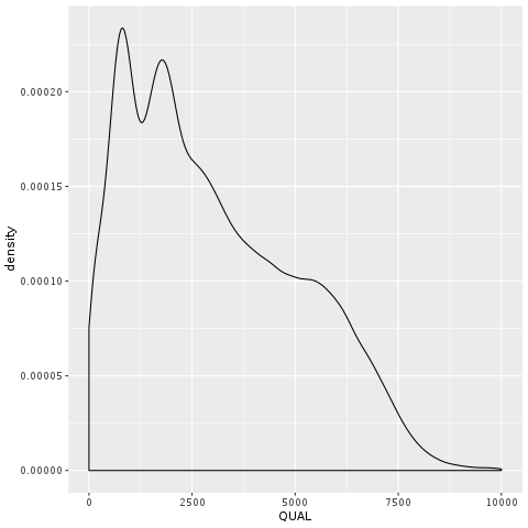
Figure 2-11. Density plot of QUAL; A. All calls together; B. Stratified by callsets annotation.

You can see on the plot that most of the low-credibility calls (in grey in B) are clustering at the very low end of the QUAL range, but you also see that the distribution is very continuous; there’s not a clear separation between bad calls and good calls, limiting the usefulness of this annotation for filtering. It’s probable that the depth-driven inflation effect is still causing us trouble even at more reasonable levels of coverage. So let’s see if we can get that confounding factor out of the equation. Enter QD, for QualByDepth. The QD annotation puts the variant confidence QUAL score into perspective by normalizing for the amount of coverage available, which compensates for the inflation phenomenon we noted above.

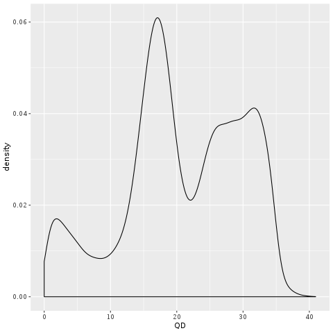
Figure 2-12. Density plot of QD; A. All calls together; B. Stratified by callsets annotation.

Even without the truth set stratification option, we already see that the shape of the density curve suggests this annotation is going to be more helpful. And indeed, when we run with the split turned on we see a clear pattern where there is more separation between “bad variants” and the rest. You see the small “shoulder” on the low end of the QD distribution? Those are all the very low-quality variant calls that are most probably junk, as confirmed by the GIAB stratification. In general, QD value tends to be a rather reliable indicator of variant call quality.

Since the various annotations measure different aspects of the variant context, it’s interesting to examine how well they might perform when combined. One way to approach this question i sto combine the scatter and density plots we’ve been making into a single figure like Figure 5-13, which shows both the two-way scatter of two annotations (here, QD and DP) and their respective density curves on the sides of the scatter plot. This provides us with some insight into how probable true variants seem to cluster within the annotation space. If nothing else, the blobs of color in the middle (which is where the “goodies” are clustering) are reasonably clearly demarcated from the grey smear of likely false positives on the left side of the plot.

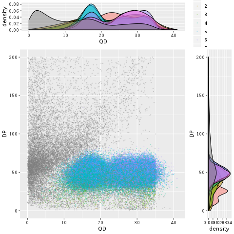
Figure 2-13. Scatter plot with marginal densities of QD vs. DP.

So what do we do with this insight? We use it as a guide to set thresholds with reasonable confidence on each annotation, reflecting how much each of them contributes to allowing us to weed out different subsets of false positive variants. The resulting combined filtering rule might be more powerful than the sum of its parts.

Applying hard filters to germline SNPs and indels

Looking at the plots in the previous section gave us some insight into what the variant context annotations represent and how we can use them to derive some rudimentary filtering rules. Now let’s see how we can actually apply those rules to our callset.

Earlier we looked at the QualByDepth annotation, which is captured in VCF records as QD. The plots we made showed that variants with a QD value below 2 are most likely not real, so let’s filter out sites with QD < 2 using the GATK tool VariantFiltration as follows. We give it a reference genome (-R), the VCF file of variants we want to filter (-V), and we specify an output file name (-O). In addition, we also provide a filtering expression that states what filtering logic to apply (here, QD < 2.0 means reject any variants with a QD value below 2.0) and what name to give to the filter (here, QD2).

# gatk VariantFiltration 
	-R ref/ref.fasta 
	-V vcfs/motherSNP.vcf.gz 
	--filter-expression "QD < 2.0" 
	--filter-name "QD2" 
	-O sandbox/motherSNP.QD2.vcf.gz

This produces a VCF with all the original variants; those that failed the filter are annotated with the filter name in the FILTER column.

# zcat sandbox/motherSNP.QD2.vcf.gz | grep -v '##' | head -3
#CHROM  POS     ID      REF     ALT     QUAL    FILTER  INFO    FORMAT  NA12878
20      61098   .       C       T       465.13  PASS    AC=1;AF=0.500;AN=2;BaseQRankSum=0.516;ClippingRankSum=0.00;DP=
44;ExcessHet=3.0103;FS=0.000;MQ=59.48;MQRankSum=0.803;QD=10.57;ReadPosRankSum=1.54;SOR=0.603    GT:AD:DP:GQ:PL  0/1:28
,16:44:99:496,0,938
20      61795   .       G       T       2034.16 PASS    AC=1;AF=0.500;AN=2;BaseQRankSum=-6.330e-01;ClippingRankSum=0.0
0;DP=60;ExcessHet=3.9794;FS=0.000;MQ=59.81;MQRankSum=0.00;QD=17.09;ReadPosRankSum=1.23;SOR=0.723        GT:AD:DP:GQ:PL
0/1:30,30:60:99:1003,0,1027

Now what if we wanted to combine filters? We could complement the QD filter by also filtering out the calls with extremely high DP since we saw those are heavily associated with false positives. We could run VariantFiltration again on the previous output with the new filter, or we could go back to the original data and apply both filters in one go like this:

# gatk VariantFiltration 
	-R ref/ref.fasta 
	-V vcfs/motherSNP.vcf.gz 
	--filter-expression "QD < 2.0 || DP > 100.0" 
	--filter-name "lowQD_highDP" 
	-O sandbox/motherSNP.QD2.DP100.vcf.gz

The double pipe (||) in the filtering expression is equivalent to a logical OR operator. You can use it any number of times, and you can also use && for the logical AND operator, but beware of building overly complex filtering queries. Sometimes it is frankly better to keep it simple and split your queries into separate components, both for clarity and for testing purposes.

The GATK hard filtering tools offer various options for tuning these commands, including deciding how to handle missing values. Keep in mind however that hard filtering is a relatively simplistic filtering technique, and it is not considered part of the GATK Best Practices. The advantage of this approach is that it is fairly intuitive if you have a good understanding of what the annotations mean and how they are calculated. In fact, it can be very effective in the hands of an expert analyst. However, it gives you a lot of dials to tune, can be overwhelming for newcomers, and tends to require new analytical work for every new project because the filtering thresholds that are appropriate for one dataset are often not directly applicable to other datasets.

We included hard filtering here because it’s an accessible way to explore what happens when you apply filters to a callset. For most “real” work we recommend applying the appropriate machine learning approaches covered in Chapter 6.

Other supported use cases

If you are interested in the following use cases, please visit the GATK website, which offers documentation for all best practice pipelines that are currently available.

• Germline copy number variation

• Structural variation

• Mitochondrial variation

• Blood biopsy

• Pathogen / contaminant identification