Chapter 2. Entity Resolution Revisited
This chapter uses entity resolution for a streaming video service as an example of unsupervised machine learning with graph algorithms. After completing this chapter, you should be able to:
-
Name the categories of graph algorithms which are appropriate for entity resolution as unsupervised learning.
-
List three different approaches for assessing the similarity of entities.
-
Understand how parameterized weights can adapt entity resolution to be a supervised learning task.
-
Interpret a simple GSQL FROM clause and have a general understanding of ACCUM semantics.
-
Set up and run a TigerGraph Cloud Starter Kit using GraphStudio.
Goal: Identify Real-World Users and Their Tastes
The streaming video on demand (SVoD) market is big business. Accurate estimates of the global market size are hard to come by, but the most conservative estimate may be $50 billion in 20201 with annual growth rates ranging from 11%2 to 21%3 for the next five years or so. Movie studios, television networks, communication networks, and tech giants have been merging and reinventing themselves, in hopes of becoming a leader in the new preferred format for entertainment consumption: on-demand digital entertainment, on any video-capable device.
To succeed, SVoD providers need to have the content to attract and retain many millions of subscribers. Traditional video technology (movie theaters and broadcast television) limited the provider to offering only one program at a time per venue or per broadcast region. Viewers had very limited choice, and providers selected content that would appeal to large segments of the public. Home video on VHS tape and DVD introduced personalization; wireless digital video on demand on any personal device has put the power in the hands of the consumer.
Providers no longer need to appeal to the masses. On the contrary, the road to success is microsegmentation: to offer something for everyone. The SVoD giants are assembling sizable catalogs of existing content, as well as spending billions of dollars on new content. The volume of options creates several data management problems. With so many shows available, it is very hard for users to browse. Providers must categorize the content, categorize users, and then recommend shows to users. Good recommendations increase viewership and satisfaction.
While predicting customers’ interests is hard enough, the streaming video industry also needs to overcome a multifaceted entity resolution problem. Entity resolution, you may recall, is the task of identifying two or more entities in a dataset which refer to the same real-world entity, and then linking or merging them together. In today’s market, streaming video providers face at least three entity resolution challenges. First, each user may have multiple different authorization schemes, one for each type of device they use for viewing. Second, corporate mergers are common, which require merging the databases of the constituent companies. For example, Disney+ combines the catalogs of Disney, Pixar, Marvel, and National Geographic Studios. HBO Max brings together HBO, Warner Bros., and DC Comics. Third, SVoD providers may form a promotional, affiliate, or partnership arrangement with another company: a customer may be able to access streaming service A because they are a customer of some other service B. For example, customers of AT&T fiber internet service may qualify for free HBO Max service.
Solution Design
Before we can design a solution, let’s start with a clear statement of the problem we want to solve.
Note
Title: Problem Statement
Each real-world user may have multiple digital identities. The goal is to discover the hidden connections between these digital identities and then to link or merge them together. By doing so, we will be able to connect all of the information together, forming a more complete picture of the user. In particular, we will know all the videos that a person has watched, in order to get a better understanding of their personal taste and to make better recommendations.
Now that we’ve crafted a clear problem statement, let’s consider a potential solution -- entity resolution. Entity resolution has two parts: deciding which entities are probably the same, and then resolving entities. Let’s look at each part in turn.
Learning Which Entities Are The Same
If we are fortunate enough to have training data showing us examples of entities that are in fact the same, we can use supervised learning to train a machine learning model. In this case, we do not have training data. Instead, we will rely on the characteristics of the data itself, looking at similarities and communities to perform unsupervised learning.
To do a good job, we want to build in some domain knowledge. What are the situations for a person to have multiple online identities, and what would be the clues in the data? Here are some reasons why a person may create multiple accounts:
-
A user creates a second account because they forgot about or forgot how to access the first one.
-
A user has accounts with two different streaming services, and the companies enter a partnership or merge.
-
A person may intentionally set up multiple distinct identities, perhaps to take advantage of multiple membership rewards or to separate their behavioral profiles (e.g., to watch different types of videos on different accounts). The personal information may be very different, but the device IDs might be the same.
Whenever the same person creates two different accounts at different moments, there can be variations in some details for trivial or innocuous reasons. The person decides to use a nickname. They choose to abbreviate a city or street name. They mistype. They have multiple phone numbers and email addresses to choose from, and they make a different choice for no particular reason. Over time, more substantial changes may occur, to address, phone number, device IDs, and even to the user’s name.
While several situations can result in one person having multiple online identities, it seems we can focus our data analysis on only two patterns. In the first pattern, most of the personal information will be the same or similar, but a few attributes may differ. Even when two attributes differ, they may still be related, such as use of a nickname or a misspelling of an address. In the second pattern, much of the information is different, but one or more key pieces remain the same, such as home phone number or birthdate, and behavioral clues (such as what type of videos they like and what time of day do they watch them) may suggest that two identities belong to the same person.
To build our solution, we will need to use some similarity algorithms and also a community detection or clustering algorithm to group similar entities together.
Resolving Entities
Once we have used the appropriate algorithms to identify a group of entities that we believe to be the same, what will do about it? We want to update the database somehow to reflect this new knowledge. There are two possible ways to accomplish this: merge the group into one entity or link the entities in a special way so that whenever we look at one member of the group, we will readily see the other related identities.
Merging the entities makes sense only when some online identities are considered incorrect, so we want to eliminate them. For example, suppose a customer has two online accounts because they misspelled their name or forgot that they had an account already. Both the business owner and the customer wants to eliminate one account and to merge all of the records (purchase history, game scores, etc.) into one account. Knowing which account to eliminate takes more knowledge of each specific case than we have in our example.
We will take the safer route and simply link entities together. Specifically, we will have two types of entities in the graph: one representing digital identities and the other representing real-world entities. After resolution, the database will show one real-world entity having an edge to each of its digital identities, as illustrated in Figure 2-1.

Figure 2-1. Digital entities linked to a real-world entity, after resolution
Implementation
The implementation of graph-based entity resolution we present below is available as a TigerGraph Cloud Starter Kit. As usual, we will focus on using the GraphStudio visual interface. All of the necessary operations could also be performed from a command line interface, but that would lack the visual interface.
Starter Kit
To get and install your Starter Kit, do one of the following::
-
Use a TigerGraph Cloud instance preloaded with this example, go to tgcloud.io and select the Starter Kit called In-Database Machine Learning for Big Data Entity Resolution.
-
Load this Starter Kit onto your own machine which is running TigerGraph, either on-premises or on the cloud, go to www.tigergraph.com/starterkits.
-
Find In-Database Machine Learning for Big Data Entity Resolution.
-
Download Data Set and the solution package corresponding to your version of the TigerGraph platform.
-
Start your TigerGraph instance. Go to the GraphStudio home page.
-
Click Import An Existing Solution, as highlighted in Figure 2-2, and select the solution package which you downloaded
-
Warning
Importing a GraphStudio Solution will delete your existing database. If you wish to save your current design, perform a GraphStudio Export Solution and also gsql backup.
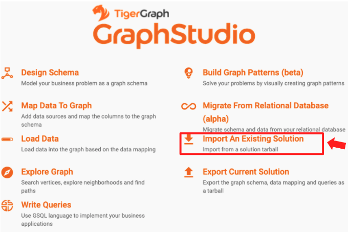
Figure 2-2. Importing a GraphStudio solution
Graph Model
The Starter Kit is preloaded with a graph model based on an actual SVoD business. The name of the graph is Entity_Resolution. When you start GraphStudio, you are working at the global graph view. To switch to the Entity_Resolution graph, click on the circular icon in the upper left corner. A dropdown menu will appear, showing you the available graphs and letting you create a new graph. Click on Entity_Resolution.
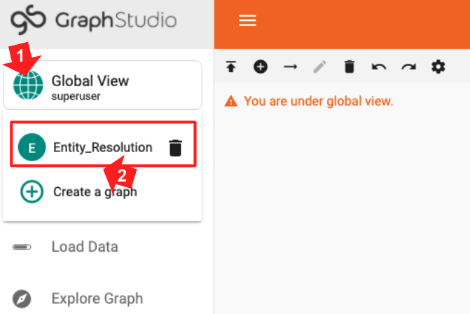
Figure 2-3. Selecting the graph to use
You should now see a graph model or schema like the one in Figure 2-4 in the main display panel.
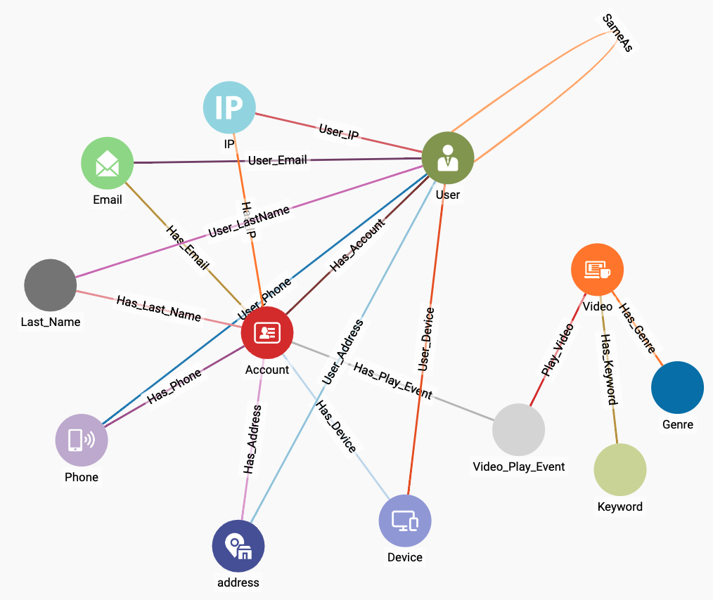
Figure 2-4. Graph schema for video customer accounts
You can see that Account, User, and Video are hub vertices with several edges radiating from them. The other vertices represent the personal information about users and the characteristics of videos. We want to compare the personal information of different users. Following good practice for graph-oriented analytics, if we want to see if two or more entities have something feature in common, e.g., email address, we model that feature as a vertex instead of as a property of a vertex. Table 2-1 gives a brief explanation of each of the vertex types in the graph model. Though the starter kit’s data contains much data about videos, we will not focus on the videos themselves in this exercise. We are going to focus on entity resolution of Accounts.
| Account | an account for a SVoD user, a digital identity |
| User | a real-world person. One User can link to multiple Accounts |
| IP, Email, Last_User, Phone, Address, Device | attributes of an Account. They are represented as vertices instead of internal properties of Account to facilitate linking Accounts/Users that share a common attribute. |
| Video | a video title offered by an SVoD |
| Keyword, Genre | attributes of a Video |
| Video_Play_Event | the time and duration of a particular Account viewing a particular Video |
Data Loading
In TigerGraph Starter Kits, the data is included, but it is not yet loaded into the database. To load the data, switch to the Load Data page (step 1 of Figure 2-5), wait a few seconds until the Load button in the upper left of the main panel becomes active, and then click it (step 2). You can watch the progress of the loading in the real-time chart at the right (not shown). Loading the 84K vertices and 270K edges should take only about 40 seconds on the TGCloud free instances; faster on the paid instances.

Figure 2-5. Loading data in a Starter Kit
Queries and Analytics
We will analyze the graph and run graph algorithms by composing and executing queries in GSQL, TigerGraph’s graph query language. When you first deploy a new Starter Kit, you need to install the queries. Switch to the Write Queries page (step 1 of Figure 2-6). Then at the top right of the list of queries, click the Install All icon (step 2).

Figure 2-6. Installing queries
For our entity resolution use case, we have a three-stage plan requiring three or more queries.
- Initialization
-
For each
Accountvertex, create its ownUservertex and link them. Accounts are online identities, and Users represent real-world persons. We begin with the hypothesis that eachAccountis a real person. - Similarity Detection
-
Apply one or more similarity algorithms to measure the similarity between
Uservertices. If we consider a pair to be similar enough, then we create a link between them, using theSameAsedge type shown in Figure 2-5. - Merging
-
Find the connected components of linked User vertices. Pick one of them to be the main vertex. Transfer all of the edges of the other members of the community to the main vertex. Delete the other community vertices.
For reasons we will explain when we talk about merging, you may need to repeat steps 2 and 3 as a pair, until the Similarity Detection step is no longer creating any new connections.
We will present two different methods for implementing entity resolution in our use case. The first method uses Jaccard similarity (introduced in Chapter 10) to count exact matches of neighboring vertices. Merging will use a Connected Component algorithm. The second method is a little more advanced, suggesting a way to handle both exact and approximate matches of attribute values. Approximate matches are a good way to handle minor typos or the use of abbreviated names.
Method 1: Jaccard Similarity
For each of the three stages, we’ll give a high level explanation, directions for operations to perform in TigerGraph’s GraphStudio, what to expect as a result, and a closer look at some of the GSQL code in the queries.
Initialization
Recall in our model that an Account is a digital identity, and a User is a real person. The original database contains only Accounts. The initialization step creates a unique temporary User linked to each Account. And, for every edge from an Account to one of the attribute vertices (Email, Phone, etc.), we create a corresponding edge from the User to the same set of attribute vertices. Figure 2-7 shows an example. The three vertices on the left and the two edges connecting them are part of the original data. The initialization step creates the User vertex and the three dotted-line edges. As a result, each User starts out with the same attribute neighborhood as its Account.
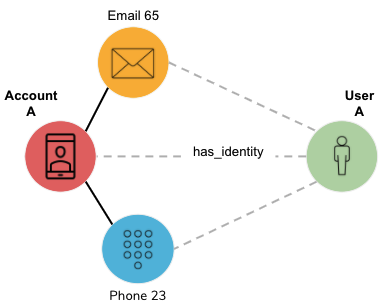
Figure 2-7. User vertex and edges created in the initialization step
Run the GSQL query initialize_users by selecting the query name from the list (step 1 in Figure 2-8) and then clicking the Run icon above the code panel (step 2). This query has no input parameters, so it will run immediately without any additional steps from the user.
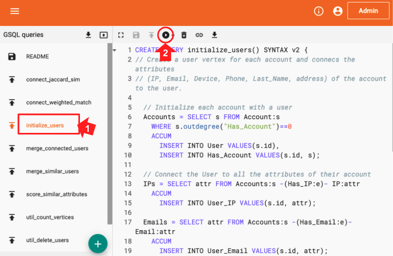
Figure 2-8. Running the initialize_users query
Let’s take a look at the GSQL code. The block of code below shows the first 20 lines of initialize_users. If you are familiar with SQL, then GSQL may look familiar. The comment at the beginning (lines 2 and 3) lists the 6 types of attribute vertices to be included. Lines 6 to 10 create a User vertex (line 9) and an edge connecting the User to the Accounts (line 10) for each Account (line 6) which doesn’t already have a neighboring User (line 7).
1   CREATE QUERY initialize_users() SYNTAX v2 {
2   // Create a User vertex for each Account, plus edges to connect attributes
3   // (IP, Email, Device, Phone, Last_Name, Address) of the Account to the User
4
5   // Initialize each account with a user
6   Accounts = SELECT s FROM Account:s
7   WHERE s.outdegree("Has_Account")==0
8   ACCUM
9     INSERT INTO User VALUES(s.id),
10    INSERT INTO Has_Account VALUES(s.id, s);
11
12  // Connect the User to all the attributes of their account
13  IPs = SELECT attr FROM Accounts:s -(Has_IP:e)- IP:attr
14  ACCUM
15    INSERT INTO User_IP VALUES(s.id, attr);
16
17  Emails = SELECT attr FROM Accounts:s -(Has_Email:e)- Email:attr
18  ACCUM
19    INSERT INTO User_Email VALUES(s.id, attr);
20  // Remaining code omitted for brevity
21  }
Tip
GSQL’s ACCUM clause is an iterator with parallel asynchronous processing. Think of it as “FOR EACH set of vertices and edges which match the pattern in the FROM clause, do the following.”
Lines 13 to 15 take care of IP attribute vertices: If there is a Has_IP edge from an Account to an IP vertex, then insert an edge from the corresponding User vertex to the same IP vertex. While the alias s defined in line 13 refers to an Account, s.id in line 15 can refer to a User because the source vertex of a User_IP edge may only be a User, and we recently used s.id to create a User (line 9). Lines 17 to 19 take care of Email attribute vertices in an analogous way. The code blocks for the remaining four attribute types (Device, Phone, Last_Name, and Address) have been omitted for brevity.
Similarity Detection
Jaccard similarity counts how many attributes two entities have in common, divided by the total number of attributes between them. Each comparison of attributes results in a yes/no answer; a miss is as good as a mile. Figure 2-9 shows an example where User A and User B each have three attributes; two of those match (Email 65 and Device 87). Therefore, A and B have two attributes in common.
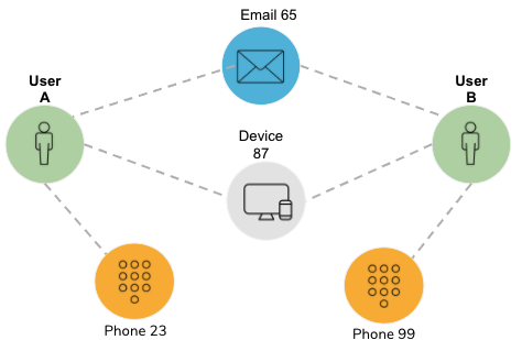
Figure 2-9. Jaccard similarity example
They have a total of four distinct attributes (Email 65, Device 87, Phone 23, and Phone 99); therefore, the Jaccard similarity is 2/4 = 0.5.
Do: Run connect_jaccard_sim.
The query connect_jaccard_sim computes this similarity score for each pair of vertices. If the score is at or above the given threshold, then create a Same_As edge to connect the two Users. The default threshold is 0.5, but you can make it higher or lower. Jaccard scores range from 0 to 1. Figure 2-10 shows the connections for User vertices 1, 2, 3, 4, and 5, using Jaccard similarity and a threshold of 0.5. For these five vertices, we need communities that range in size from one vertex alone (User 3) to two clusters of three (Users 1 and 2).

Figure 2-10. Connections for User vertices 1, 2, 3, 4, and 5, using Jaccard similarity and a threshold of 0.5
Rather than showing the full code, we’ll just focus on a few excerpts. In the first code snippet, we’ll show how to count the attributes in common between every pair of Users, using a single SELECT statement. The statement uses pattern-matching to describe how two such Users would be connected, and then it uses an accumulator to count the occurrences.
1   Others = SELECT B FROM
2   Start:A -()- (IP|Email|Phone|Last_Name|Address|Device):n -()- User:B
3   WHERE B != A
4   ACCUM
5     A.@intersection += (B -> 1); // tally each path A->B,
6     @@path_count += 1            // count the total number of paths
Note
GSQL’s FROM clause describes a left-to-right path moving from vertex to vertex via edges. Each sequence of vertices and edges which fit the requirements form one “row” in the temporary “table” of results, which is passed on to the ACCUM and POST-ACCUM clauses for further processing.
The FROM clause in lines 1 to 2 presents a graph path pattern to search for. FROM User:A -()- (IP|Email|Phone|Last_Name|Address|Device):n -()- User:B defines a two-hop path pattern:
-
User:Ameans start from a User vertex, aliased toA, -
-()-means pass through any edge type -
(IP|Email|Phone|Last_Name|Address|Device):nmeans arrive at one of these six vertex types, aliased ton -
-()-means pass through another edge of any type, and finally -
User:Bmeans arrive at a User vertex, aliased toB
In line 3, (WHERE B != A) ensures that we skip the situation of a loop where A = B. Line 4 announces the start of an ACCUM clause. Line 5 (A.@intersection += (B -> 1); // tally each path A->B) is a good example of GSQL’s support for parallel processing and aggregation: for each path from A to B, append a key → value record attached to A. The record is (B, +=1). That is, if this is the first record associating B with A, then set the value to 1. For each additional record where B is A’s target, then increment the value by 1. Hence, we’re counting how many times there is a connection from A to B, via one of the six specified edge types. Line 6 (ACCUM @@path_count += 1) is just for bookkeeping purposes, to count now many of these paths we find.
Let’s look at one more code block, the final computation of Jaccard similarity and creation of connections between Users.
1   Result = SELECT A FROM User:A
2   ACCUM FOREACH (B, overlap) IN A.@intersection DO
3   FLOAT score = overlap*1.0/(@@deg.get(A) + @@deg.get(B) - overlap),
4   IF score > threshold THEN
5     INSERT INTO EDGE SameAs VALUES (A, B, score), // FOR Entity Res
6     @@insert_count += 1,
7     IF score != 1 THEN
8       @@jaccard_heap += SimilarityTuple(A,B,score)
9     END
10  END
11  END;
This SELECT block does the following:
-
For each User A, iterate over its record of similar Users B and the number of common neighbors, aliased to
overlap. -
For each such pair (A, B), compute the Jaccard score, using
overlapas well as the number of qualified neighbors of A and B (@@deg.get(A)and@@deg.get(B)), computed earlier. -
If the score is greater than the threshold, insert a SameAs edge between A and B.
-
@@insert_countand@@jaccard_heapare for reporting statistics and are not essential.
Merging
In our third and last stage, we merge together the connected communities of User vertices which we created in the previous step. For each community, we will select one vertex to be the survivor or lead. The remaining members will be deleted; all of the edges from an Account to a non-lead will be redirected to point to the lead User.
Do: run query merge_connected_users. Look at the JSON output. Note whether t says converged = TRUE or FALSE.
Figure 2-13 displays the User communities for Accounts 1, 2, 3, 4, and 5. The user communities have been reduced to a single User (real person). Each of those Users links to one or more Accounts (digital identities). We’ve achieved our entity resolution.

Figure 2-13. Entity resolution achieved, using Jaccard similarity
The merge_connected_users algorithm has four stages:
-
Find connected users using the connected component algorithm.
-
In each component, select a lead user.
-
In each component, redirect the attribute connections from other users to the lead user.
-
Delete the users that are not the lead user and all of the Same_As edges.
We’ll take a closer look at the GSQL code for the Connected Components algorithm.
1   Users = {User.*};
2   Updated_users = SELECT s FROM Users:s
3     POST-ACCUM
4       s.@min_user_id = s;
5
6   WHILE (Updated_users.size() > 0) DO
7     IF verbose THEN PRINT iteration, Updated_users.size(); END;
8     Updated_users = SELECT t
9      FROM Updated_users:s -(SameAs:e)- User:t
10      // Propagate the internal IDs from source to target vertex
11     ACCUM t.@min_user_id += s.@min_user_id   // t gets the lesser of t & s ids
12     HAVING t.@min_user_id != t.@min_user_id' // accum is accum's previous val
13      ;
14    iteration = iteration + 1;
15  END;
Line 1 initializes the vertex set called Users to be all User vertices. Lines 2 to 4 initializes an accumulator variable @min_user_id for each User. The initial value is the vertex’s internal ID (different from the externally visible ID). This variable will store the algorithm’s current best guess at the community ID for this vertex: all vertices having the same value of @min_user_id belong to the same community. It’s important to note that this accumulator is a MinAccum. Whenever you input a new value to a MinAccum, it retains the lesser of its current value and the new input value.
Lines 8 to 11 says that for each connected User pair from s to t, set t.@min_user_id to the lesser of s and t’s community IDs. Line 12 says that the output set (Updated_users in line 8) should contain only those User vertices who updated their community ID in this round. Note the tick mark ' at the end of the line; this is actually a modifier for the accumulator t.@min_user_id. It means “the previous value of the accumulator”; this lets us easily compare the previous to current values. When no vertices have changed their ID, then we can exit the WHILE loop (line 6).
Are We There Yet?
It might seem that one pass through the three steps – initialize, connect similar entities, and merge connected entities – should be enough. The merging, however, can create a situation in which new similarities arise. Take a look at Figure 2-14, which depicts the attribute connections of User 302 after Users 2 and 602 have been merged into it. Accounts 2, 302, and 602 remain separate, so you can see how each of them contributed some attributes. Because User 302 has more attributes than before, it is now possible that it is more similar than before to some other (possibly newly merged) User. Therefore, we should run another round of similarity connection and merge. Repeat these steps until no new similarities arise.
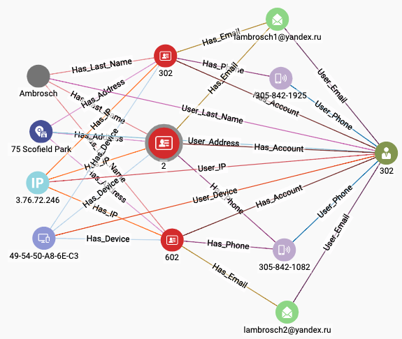
Figure 2-14. User with more attributes after entity resolution
Note
For convenient reference, here is the sequence of queries we ran for simple entity resolution using Jaccard similarity:
Run initialize_users
Run connect_jaccard_sim
Run merge_connected_users
Repeat steps 2 & 3 until the output of merge_connected_users says conversed = TRUE
Reset
After you’ve finished, or at any time, you might want to restore the database to its original state. You need to do this if you want to run the entity resolution process from the start again. The query util_delete_users will delete all User vertices and all edges connecting to them. Note that you need to change the input parameter are_you_sure from FALSE to TRUE. This manual effort is put in as a safety precaution.
Warning
Deleting bulk vertices (util_delete_users) or creating bulk vertices (initialize_users) can take tens of seconds in the modestly sized free TigerGraph Cloud instances. Go to the Load Data page to check the live statistics for User vertices and User-related edges to see if the creation or deletion has finished.
Method 2: Scoring Exact and Approximate Matches
The previous section demonstrated a nice and easy graph-based entity resolution technique, but it is too basic for real-world use. It relies on exact matching of attribute values, whereas we need to allow for almost-the-same values, which arise from unintentional and intentional spelling variations. We also would like to make some attributes more important than others. For example, if you happen to have date-of-birth information, you might be strict about this attribute matching exactly. While persons can move, have multiple phone numbers and email addresses, they can only have one birthdate. In this section, we will introduce weights to adjust the relative importance of different attributes. We will also provide a technique for approximate matches of string values.
Note
If you already used your starter kit to run Method 1, be sure to reset it. (See the Reset section at the end of Method 1.)
Initialization
We are still using the same graph model with User vertices representing real persons and Account vertices representing digital accounts. So, we are still using the initialize_users query to set up an initial set of User vertices.
We are adding another initialization step. We are going to assign weights to each of the six attributes: IP, Email, Phone, Address, Last_Name, and Device. If this were a relational database, we would store those weights in a table. Since this is a graph, we are going to store them in a vertex. We only need one vertex, because one vertex can have multiple attributes. However, we are going to be even more fancy. We are going to use a map type attribute, which will have six key → value entries. This allows us to use the map like a lookup table: tell me the name of the key (attribute name), and I’ll tell you the value (weight).
Do:
-
Run initialize_users. Check the graph statistics on the Load Data page to make sure that all 900 Users and related edges have been created.
-
Run util_set_weights. The weights for the six attributes are input parameters for this query. Default weights are included, but you may change them if you wish. If you want to see the results, run util_print_vertices.
Scoring Weighted Exact Matches
We are going to do our similarity comparison and linking in two phases. In phase one, we are still checking for exact matches because exact matches are more valuable than approximate matches; however, those connections will be weighted. In phase two, we will then check for approximate matches for our two attributes which have alphabetic values: Last_Name and Address.
In weighted exact matching, we create weighted connections between Users, where higher weights indicate stronger similarity. The net weight of a connection is the sum of the contributions from each attribute that is shared by the two Users. Figure 2-15 illustrates the weighted match computation. Earlier, during the initialization phase, you established weights for each of the attributes of interest. In the figure, we use the names wt_email and wt_phone for the weights associated with matching Email and Phone attributes, respectively.
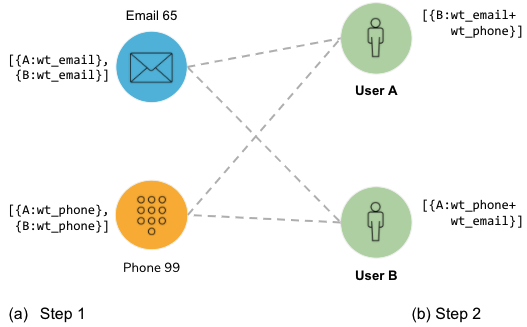
Figure 2-15. Two-phase calculation of weighted matches
The weighted match computation has two steps. In step 1, we look for connections from Users to Attributes and record a weight on each attribute for a connection to each User. Both User A and User B connect to Email 65, so Email 65 records A:wt_email and B:wt_email. Each User’s weight needs to be recorded separately. Phone 99 also connects to Users A and B so it records analogous information.
In step 2, we look for the same connections but in the other direction, with Users as the destinations. Both Email 65 and Phone 99 have connections to User A. User A aggregates their records from step 1. Note that some of those records refer to User A. User A ignores those, because it is not interested in connections to itself! In this example, it ends up recording B:(wt_email + wt_phone). We use this value to create a weighted Same_As edge between Users A and B. You can see that User B has equivalent information about User A.
Do: run connect_weighted_match.
Figure 2-16 shows one of the communities generated by connect_weighted_match. This particular community is the one containing User/Account 5. The figure also shows connections to two attributes, Address and Last_Name. The other attributes such as Email were used in the scoring but are not shown, to avoid clutter.
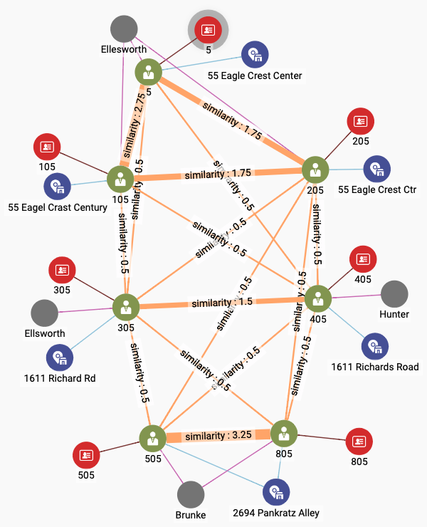
Figure 2-16. User community including Account 5 after exact weighted matching
The thickness of the SameAs edges indicates the strength of the connection. The strongest connection is between Users 505 and 805 at the bottom of the screen. In fact, we can see three subcommunities of Users among the largest community of seven members:
-
Users 5, 105, and 205 at the top. The bond between Users 5 and 105 is a little stronger, for reasons not shown. All three share the same last name. They have similar addresses.
-
Users 305 and 405 in the middle. Their last names and address are different, so some of the attributes not shown must be the cause of their similarity.
-
Users 505 and 805 at the bottom. They share the same last name and address, as well as other attributes.
Scoring Approximate Matches
We can see (in Figure 2-16) that some Users have similar names (Ellsworth vs. Ellesworth) and similar addresses (Eagle Creek Center vs. Eagle Crest Ctr). A scoring system that looks only for exact matchings gives us no credit for these near misses. An entity resolution system would like to be able to assess the similarity of two text strings and to assign a score to the situation. Do they differ by a single letter, like Ellsworth and Ellsworth? Are letters transposed, like Center and Cneter? Computer scientists like to think of the edit distance between two text strings: how many single-letter changes of value or position are needed to transform string X into string Y?
We are going to use the Jaro-Winkler similarity to measure the similarity between two strings, an enhancement of Jaro similarity. Given two strings s1 and s2, who have m matching characters and t transformation steps between them, then their Jaro similarity is defined as shown in Equation 2-1.
Equation 2-1. Definition of Jaro similarity
If the strings are identical, then m = |s1| = |s2|, and t =0, so the equation simplifies to (1 + 1 + 1)/3 = 1. On the other hand, if there are no letters in common, then the score = 0. We then multiply this score by the weight for the attribute type. For example, if the attribute’s weight is 0.5, and if the JaroWinkler similarity score is 0.9, then the net score is 0.5 * 0.9 = 0.45.
Jaro-Winkler similarity takes Jaro as a starting point and adds an additional reward if the beginnings of each string, reading from the left end, match exactly.
Do: Run score_similar_attributes.
The score_similar_attributes query considers the User pairs which already are linked by a Same_As edge. It computes the weighted Jaro-Winkler similarity for the Last_Name and the Address attributes, and adds those scores to the existing similarity score. We chose Last_Name and Address because they are alphabetic instead of numeric. This is an application decision rather than a technical one. Figure 2-17 shows the results after adding in the scores for the approximate matches.

Figure 2-17. User community including Account 5 after exact and approximate weighted matching
Comparing Figures 11-16 and 11-17, we notice the following changes:
-
The connections among Users 1, 105, and 205 have strengthened due to their having similar addresses.
-
User 305 is more strongly connected to the trio above due to a similar last name.
-
The connection between 305 and 405 has strengthened due to their having similar addresses.
-
User 405 is more strongly connected to Users 505 and 805 due to the name Hunter having some letters in common with Brunke. This last effect might be considered an unintended consequence of the Jaro-Winkler similarity measure not being as judicious as a human evaluator would be.
Comparing two strings is a general purpose function which does not require graph traversal, so we have implemented it as a simple string function in GSQL. Because it is not yet a built-in feature of the GSQL language, we took advantage of GSQL’s ability to accept a user-supplied C++ function as a user-defined function (UDF). The UDFs for jaroDistance(s1, s2) and jaroWinklerDistance(s1, s2) are included in this starter kit. You can invoke them from within a GSQL query anywhere that you would be able to call a built-in string function.
The code snippet below shows how we performed the approximate matching and scoring for the Address feature:
1   Connected_users = SELECT A
2     // Find all linked users, plus each user's address
3     FROM Connected_users:A -(SameAs:e)- User:B,
4        User:A -()- Address:A_addr,
5        User:B -()- Address:B_addr
6     WHERE A.id < B.id    // filter so we don't count (A,B) & (B,A)
7     ACCUM @@addr_match += 1,
8     // If addresses aren't identical compute JaroWinkler * weight
9     IF do_address AND A_addr.val != B_addr.val THEN
10      FLOAT sim = jaroWinklerDistance(A_addr.id,B_addr.id) * addr_wt,
11      @@sim_score += (A -> (B -> sim)),
12      @@string_pairs += String_pair(A_addr.id, B_addr.id),
13      IF sim != 0 THEN @@addr_update += 1 END
14    END
15  ;
Lines 3 to 5 are an example of a conjunctive path pattern, that is, a compound pattern comprising several individual patterns, separated by commas. The commas act like boolean AND. This conjunctive pattern means “find a User A linked to a User B, and find the Address connected to A, and find the Address connected to B.” Line 6 filters out the case where A = B and prevents a pair (A, B) from being processed twice.
Line 9 filters out the case where A and B are different but have identical addresses. If their addresses are the same, then we already gave them full credit when we ran connect_weighted_match. Line 10 computes the weighted scoring, using the jaroWinklerDistance function and the weight for Address. Line 11 stores this value in a lookup table temporarily. Lines 12 and 13 are just to record our activity, for informative output at the end.
Merging Similar Entities
In Method 1, we had a simpler scheme for deciding whether to merge two entities: if their Jaccard score was greater than some threshold, then we created a SameAs edge. The decision was made. Merge everything that has a SameAs edge. We want a more nuanced approach now. Our scoring has adjustable weights, and the SameAs edges record our scores. We can use another threshold score to decide which Users to merge.
Take another look at Figure 2-17. We can see the effect of threshold score for mergIng. If we set the threshold at 3.0, there would be only two merges in this community: (5, 105) and (505, 805). If we set it at 2.0, we will get the three communities that we spoke about earlier: (5, 105, 205), (305, 405), and (505, 805). If we set the threshold at 1.0, all seven Users will be merged into 1.
We only need to make two small changes to merge_connected_users to let the user set a threshold.
-
Add a threshold parameter to the query header:
CREATE QUERY merge_connected_users(FLOAT threshold=1.0, BOOL verbose=FALSE) -
In the connected component algorithm, add a WHERE clause to check the SameAs edge’s similarity value:
1   WHILE (Updated_users.size() > 0) DO
2     IF verbose THEN PRINT iteration, Updated_users.size(); END;
3     Updated_users = SELECT t
4       FROM Updated_users:s -(SameAs:e)- User:t
5       WHERE e.1  similarity > threshold
6         // Propagate the internal IDs from source to target vertex
7           // t gets the lesser of t & s ids
8       ACCUM t.@min_user_id += s.@min_user_id
9           // accum' is accum's previous val
10      HAVING t.@min_user_id != t.@min_user_id'
11    ;
12    iteration = iteration + 1;
13  END;
Run merge_connected_users. Pick a threshold value and see if you get the result that you expect.
Figure 2-18 shows the three different merging results for threshold values of 1.0, 2.0, and 3.0, to the community we have been following.
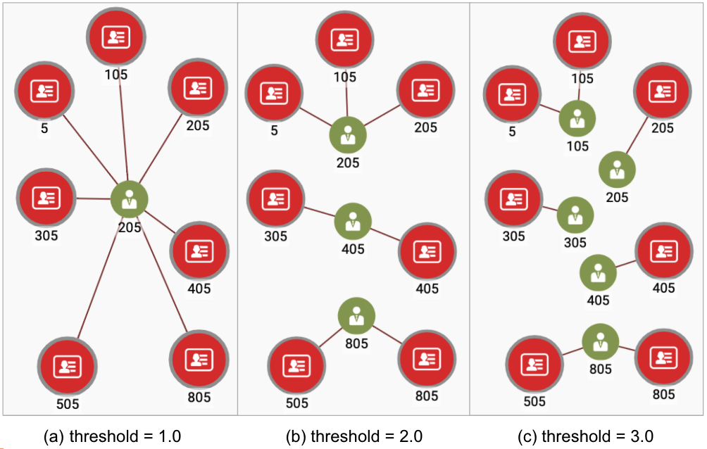
Figure 2-18. Entity resolution with different threshold levels
That concludes our second and more nuanced method of entity resolution.
Note
For convenient reference, here is the sequence of queries we ran for entity resolution using weighted exact and approximate matching:
-
Run initialize_users
-
Run util_set_weights
-
Run connect_weighed_match
-
Run score_similar_attributes
-
Run merge_connected_users
-
Repeat steps 3, 4 and 5 until the output of merge_connected_users says conversed = TRUE
Chapter Summary
In this chapter we saw how graph algorithms and other graph techniques can be used for more sophisticated entity resolution than the simple entity resolution presented earlier in this book. Similarity algorithms and the connected component algorithm play key roles. We considered several schemes for assessing the similarity of two entities: Jaccard similarity, weighted sum of exact matches, and Jaro-Winkler similarity for comparing text strings.
These approaches can readily be extended to supervised learning if training data becomes available. There are a number of model parameters that can be learned, to improve the accuracy of the entity resolution: the scoring weights of each Attribute for exact matching, tuning the scoring of approximate matches, and thresholds for merging similar Users.
We saw how we use the FROM clause in GSQL queries to select data in a graph, by expressing a path or pattern. We also saw examples of the ACCUM clause and accumulators being used to compute and store information such as the common neighbors between vertices, a tally, an accumulating score, or even an evolving ID value, marking a vertex as a member of a particular community.
This chapter showed us how graph-based machine learning can improve the ability of enterprises to see the truth behind the data. In the next chapter, we’ll apply graph machine learning to one of the most popular and important use cases: product recommendation.
1 "Video Streaming Market Report“, Grand View Research, February 2021
2 "Video Streaming (SVoD) Report“, Statista.com
3 "Video Streaming Market Report“, Grand View Research, February 2021