
Chapter 9. Modeling probabilities and nonlinearities: activation functions
What is an activation function?
Standard hidden activation functions
- Sigmoid
- Tanh
Standard output activation functions
- Softmax
Activation function installation instructions
“I know that 2 and 2 make 4—& should be glad to prove it too if I could—though I must say if by any sort of process I could convert 2 & 2 into five it would give me much greater pleasure.”
George Gordon Byron, letter to Annabella Milbanke, November 10, 1813
What is an activation function?
It’s a function applied to the neurons in a layer during prediction
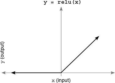
An activation function is a function applied to the neurons in a layer during prediction. This should seem very familiar, because you’ve been using an activation function called relu (shown here in the three-layer neural network). The relu function had the effect of turning all negative numbers to 0.
Oversimplified, an activation function is any function that can take one number and return another number. But there are an infinite number of functions in the universe, and not all them are useful as activation functions.
There are several constraints on what makes a function an activation function. Using functions outside of these constraints is usually a bad idea, as you’ll see.

Constraint 1: The function must be continuous and infinite in domain
The first constraint on what makes a proper activation function is that it must have an output number for any input. In other words, you shouldn’t be able to put in a number that doesn’t have an output for some reason.
A bit overkill, but see how the function on the left (four distinct lines) doesn’t have y values for every x value? It’s defined in only four spots. This would make for a horrible activation function. The function on the right, however, is continuous and infinite in domain. There is no input (x) for which you can’t compute an output (y).

Constraint 2: Good activation functions are monotonic, never changing direction
The second constraint is that the function is 1:1. It must never change direction. In other words, it must either be always increasing or always decreasing.
As an example, look at the following two functions. These shapes answer the question, “Given x as input, what value of y does the function describe?” The function on the left (y = x * x) isn’t an ideal activation function because it isn’t either always increasing or always decreasing.
How can you tell? Well, notice that there are many cases in which two values of x have a single value of y (this is true for every value except 0). The function on the right, however, is always increasing! There is no point at which two values of x have the same value of y:

This particular constraint isn’t technically a requirement. Unlike functions that have missing values (noncontinuous), you can optimize functions that aren’t monotonic. But consider the implication of having multiple input values map to the same output value.
When you’re learning in neural networks, you’re searching for the right weight configurations to give a specific output. This problem can get a lot harder if there are multiple right answers. If there are multiple ways to get the same output, then the network has multiple possible perfect configurations.
An optimist might say, “Hey, this is great! You’re more likely to find the right answer if it can be found in multiple places!” A pessimist would say, “This is terrible! Now you don’t have a correct direction to go to reduce the error, because you can go in either direction and theoretically make progress.”
Unfortunately, the phenomenon the pessimist identified is more important. For an advanced study of this subject, look more into convex versus non-convex optimization; many universities (and online classes) have entire courses dedicated to these kinds of questions.
Constraint 3: Good activation functions are nonlinear (they squiggle or turn)
The third constraint requires a bit of recollection back to chapter 6. Remember sometimes correlation? In order to create it, you had to allow the neurons to selectively correlate to input neurons such that a very negative signal from one input into a neuron could reduce how much it correlated to any input (by forcing the neuron to drop to 0, in the case of relu).
As it turns out, this phenomenon is facilitated by any function that curves. Functions that look like straight lines, on the other hand, scale the weighted average coming in. Scaling something (multiplying it by a constant like 2) doesn’t affect how correlated a neuron is to its various inputs. It makes the collective correlation that’s represented louder or softer. But the activation doesn’t allow one weight to affect how correlated the neuron is to the other weights. What you really want is selective correlation. Given a neuron with an activation function, you want one incoming signal to be able to increase or decrease how correlated the neuron is to all the other incoming signals. All curved lines do this (to varying degrees, as you’ll see).
Thus, the function shown here on the left is considered a linear function, whereas the one on the right is considered nonlinear and will usually make for a better activation function (there are exceptions, which we’ll discuss later).

Constraint 4: Good activation functions (and their derivatives) s- should be efficiently computable
This one is pretty simple. You’ll be calling this function a lot (sometimes billions of times), so you don’t want it to be too slow to compute. Many recent activation functions have become popular because they’re so easy to compute at the expense of their expressiveness (relu is a great example of this).
Standard hidden-layer activation functions
Of the infinite possible functions, which ones are most commonly used?
Even with these constraints, it should be clear that an infinite (possibly transfinite?) number of functions could be used as activation functions. The last few years have seen a lot of progress in state-of-the-art activations. But there’s still a relatively small list of activations that account for the vast majority of activation needs, and improvements on them have been minute in most cases.
sigmoid is the bread-and-butter activation
sigmoid is great because it smoothly squishes the infinite amount of input to an output between 0 and 1. In many circumstances, this lets you interpret the output of any individual neuron as a probability. Thus, people use this nonlinearity both in hidden layers and output layers.

tanh is better than sigmoid for hidden layers
Here’s the cool thing about tanh. Remember modeling selective correlation? Well, sigmoid gives varying degrees of positive correlation. That’s nice. tanh is the same as sigmoid except it’s between –1 and 1!
This means it can also throw in some negative correlation. Although it isn’t that useful for output layers (unless the data you’re predicting goes between –1 and 1), this aspect of negative correlation is powerful for hidden layers; on many problems, tanh will outperform sigmoid in hidden layers.

Standard output layer activation functions
Choosing the best one depends on what you’re trying to predict
It turns out that what’s best for hidden-layer activation functions can be quite different from what’s best for output-layer activation functions, especially when it comes to classification. Broadly speaking, there are three major types of output layer.
Configuration 1: Predicting raw data values (no activation function)
This is perhaps the most straightforward but least common type of output layer. In some cases, people want to train a neural network to transform one matrix of numbers into another matrix of numbers, where the range of the output (difference between lowest and highest values) is something other than a probability. One example might be predicting the average temperature in Colorado given the temperature in the surrounding states.
The main thing to focus on here is ensuring that the output nonlinearity can predict the right answers. In this case, a sigmoid or tanh would be inappropriate because it forces every prediction to be between 0 and 1 (you want to predict any temperature, not just between 0 and 1). If I were training a network to do this prediction, I’d very likely train the network without an activation function on the output.
Configuration 2: Predicting unrelated yes/no probabilities (sigmoid)
You’ll often want to make multiple binary probabilities in one neural network. We did this in the “Gradient descent with multiple inputs and outputs” section of chapter 5, predicting whether the team would win, whether there would be injuries, and the morale of the team (happy or sad) based on the input data.
As an aside, when a neural network has hidden layers, predicting multiple things at once can be beneficial. Often the network will learn something when predicting one label that will be useful to one of the other labels. For example, if the network got really good at predicting whether the team would win ballgames, the same hidden layer would likely be very useful for predicting whether the team would be happy or sad. But the network might have a harder time predicting happiness or sadness without this extra signal. This tends to vary greatly from problem to problem, but it’s good to keep in mind.
In these instances, it’s best to use the sigmoid activation function, because it models individual probabilities separately for each output node.
Configuration 3: Predicting which-one probabilities (softmax)
By far the most common use case in neural networks is predicting a single label out of many. For example, in the MNIST digit classifier, you want to predict which number is in the image. You know ahead of time that the image can’t be more than one number. You can train this network with a sigmoid activation function and declare that the highest output probability is the most likely. This will work reasonably well. But it’s far better to have an activation function that models the idea that “The more likely it’s one label, the less likely it’s any of the other labels.”
Why do we like this phenomenon? Consider how weight updates are performed. Let’s say the MNIST digit classifier should predict that the image is a 9. Also say that the raw weighted sums going into the final layer (before applying an activation function) are the following values:

The network’s raw input to the last layer predicts a 0 for every node but 9, where it predicts 100. You might call this perfect. Let’s see what happens when these numbers are run through a sigmoid activation function:
![]()
Strangely, the network seems less sure now: 9 is still the highest, but the network seems to think there’s a 50% chance that it could be any of the other numbers. Weird! softmax, on the other hand, interprets the input very differently:
![]()
This looks great. Not only is 9 the highest, but the network doesn’t even suspect it’s any of the other possible MNIST digits. This might seem like a theoretical flaw of sigmoid, but it can have serious consequences when you backpropagate. Consider how the mean squared error is calculated on the sigmoid output. In theory, the network is predicting nearly perfectly, right? Surely it won’t backprop much error. Not so for sigmoid:
![]()
Look at all the error! These weights are in for a massive weight update even though the network predicted perfectly. Why? For sigmoid to reach 0 error, it doesn’t just have to predict the highest positive number for the true output; it also has to predict a 0 everywhere else. Where softmax asks, “Which digit seems like the best fit for this input?” sigmoid says, “You better believe that it’s only digit 9 and doesn’t have anything in common with the other MNIST digits.”
The core issue: Inputs have similarity
Different numbers share characteristics. It’s good to let the net- twork believe that
MNIST digits aren’t all completely different: they have overlapping pixel values. The average 2 shares quite a bit in common with the average 3.
Why is this important? Well, as a general rule, similar inputs create similar outputs. When you take some numbers and multiply them by a matrix, if the starting numbers are pretty similar, the ending numbers will be pretty similar.

Consider the 2 and 3 shown here. If we forward propagate the 2 and a small amount of probability accidentally goes to the label 3, what does it mean for the network to consider this a big mistake and respond with a big weight update? It will penalize the network for recognizing a 2 by anything other than features that are exclusively related to 2s. It penalizes the network for recognizing a 2 based on, say, the top curve. Why? Because 2 and 3 share the same curve at the top of the image. Training with sigmoid would penalize the network for trying to predict a 2 based on this input, because by doing so it would be looking for the same input it does for 3s. Thus, when a 3 came along, the 2 label would get some probability (because part of the image looks 2ish).
What’s the side effect? Most images share lots of pixels in the middle of images, so the network will start trying to focus on the edges. Consider the 2-detector node weights shown at right.
See how muddy the middle of the image is? The heaviest weights are the end points of the 2 toward the edge of the image. On one hand, these are probably the best individual indicators of a 2, but the best overall is a network that sees the entire shape for what it is. These individual indicators can be accidentally triggered by a 3 that’s slightly off-center or tilted the wrong way. The network isn’t learning the true essence of a 2 because it needs to learn 2 and not 1, not 3, not 4, and so on.

We want an output activation that won’t penalize labels that are similar. Instead, we want it to pay attention to all the information that can be indicative of any potential input. It’s also nice that a softmax’s probabilities always sum to 1. You can interpret any individual prediction as a global probability that the prediction is a particular label. softmax works better in both theory and practice.
softmax computation
softmax raises each input value exponentially and then divides by- y the layer’s sum
Let’s see a softmax computation on the neural network’s hypothetical output values from earlier. I’ll show them here again so you can see the input to softmax:

To compute a softmax on the whole layer, first raise each value exponentially. For each value x, compute e to the power of x (e is a special number ~2.71828...). The value of e^x is shown on the right.

Notice that it turns every prediction into a positive number, where negative numbers turn into very small positive numbers, and big numbers turn into very big numbers. (If you’ve heard of exponential growth, it was likely talking about this function or one very similar to it.)

In short, all the 0s turn to 1s (because 1 is the y intercept of e^x), and the 100 turns into a massive number (2 followed by 43 zeros). If there were any negative numbers, they turned into something between 0 and 1. The next step is to sum all the nodes in the layer and divide each value in the layer by that sum. This effectively makes every number 0 except the value for label 9.
![]()
The nice thing about softmax is that the higher the network predicts one value, the lower it predicts all the others. It increases what is called the sharpness of attenuation. It encourages the network to predict one output with very high probability.
To adjust how aggressively it does this, use numbers slightly higher or lower than e when exponentiating. Lower numbers will result in lower attenuation, and higher numbers will result in higher attenuation. But most people just stick with e.
Activation installation instructions
How do you add your favorite activation function to any layer?
Now that we’ve covered a wide variety of activation functions and explained their usefulness in hidden and output layers of neural networks, let’s talk about the proper way to install one into a neural network. Fortunately, you’ve already seen an example of how to use a nonlinearity in your first deep neural network: you added a relu activation function to the hidden layer. Adding this to forward propagation was relatively straightforward. You took what layer_1 would have been (without an activation) and applied the relu function to each value:
layer_0 = images[i:i+1]
layer_1 = relu(np.dot(layer_0,weights_0_1))
layer_2 = np.dot(layer_1,weights_1_2)
There’s a bit of lingo here to remember. The input to a layer refers to the value before the nonlinearity. In this case, the input to layer_1 is np.dot(layer_0,weights_0_1). This isn’t to be confused with the previous layer, layer_0.
Adding an activation function to a layer in forward propagation is relatively straightforward. But properly compensating for the activation function in backpropagation is a bit more nuanced.
In chapter 6, we performed an interesting operation to create the layer_1_delta variable. Wherever relu had forced a layer_1 value to be 0, we also multiplied the delta by 0. The reasoning at the time was, “Because a layer_1 value of 0 had no effect on the output prediction, it shouldn’t have any impact on the weight update either. It wasn’t responsible for the error.” This is the extreme form of a more nuanced property. Consider the shape of the relu function.
The slope of relu for positive numbers is exactly 1. The slope of relu for negative numbers is exactly 0. Modifying the input to this function (by a tiny amount) will have a 1:1 effect if it was predicting positively, and will have a 0:1 effect (none) if it was predicting negatively. This slope is a measure of how much the output of relu will change given a change in its input.
Because the purpose of delta at this point is to tell earlier layers “make my input higher or lower next time,” this delta is very useful. It modifies the delta backpropagated from the following layer to take into account whether this node contributed to the error.
Thus, when you backpropagate, in order to generate layer_1_delta, multiply the backpropagated delta from layer_2 (layer_2_delta.dot(weights_1_2.T)) by the slope of relu at the point predicted in forward propagation. For some deltas the slope is 1 (positive numbers), and for others it’s 0 (negative numbers):
error += np.sum((labels[i:i+1] - layer_2) ** 2)

correct_cnt += int(np.argmax(layer_2) ==
                                np.argmax(labels[i:i+1]))

layer_2_delta = (labels[i:i+1] - layer_2)
layer_1_delta = layer_2_delta.dot(weights_1_2.T)
                            * relu2deriv(layer_1)

weights_1_2 += alpha * layer_1.T.dot(layer_2_delta)
weights_0_1 += alpha * layer_0.T.dot(layer_1_delta)

def relu(x):
    return (x >= 0) * x       1

def relu2deriv(output):
    return output >= 0        2
- 1 Returns x if x > 0; returns 0 otherwise
- 2 Returns 1 for input > 0; returns 0 otherwise
relu2deriv is a special function that can take the output of relu and calculate the slope of relu at that point (it does this for all the values in the output vector). This begs the question, how do you make similar adjustments for all the other nonlinearities that aren’t relu? Consider relu and sigmoid:

The important thing in these figures is that the slope is an indicator of how much a tiny change to the input affects the output. You want to modify the incoming delta (from the following layer) to take into account whether a weight update before this node would have any effect. Remember, the end goal is to adjust weights to reduce error. This step encourages the network to leave weights alone if adjusting them will have little to no effect. It does so by multiplying it by the slope. It’s no different for sigmoid.
Multiplying delta by the slope
To compute layer_delta, multiply the backpropagated delta by the layer’s slope
layer_1_delta[0] represents how much higher or lower the first hidden node of layer 1 should be in order to reduce the error of the network (for a particular training example). When there’s no nonlinearity, this is the weighted average delta of layer_2.
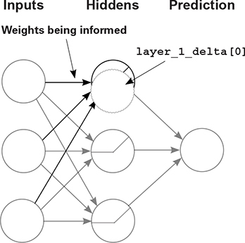
But the end goal of delta on a neuron is to inform the weights whether they should move. If moving them would have no effect, they (as a group) should be left alone. This is obvious for relu, which is either on or off. sigmoid is, perhaps, more nuanced.

Consider a single sigmoid neuron. sigmoid’s sensitivity to change in the input slowly increases as the input approaches 0 from either direction. But very positive and very negative inputs approach a slope of very near 0. Thus, as the input becomes very positive or very negative, small changes to the incoming weights become less relevant to the neuron’s error at this training example. In broader terms, many hidden nodes are irrelevant to the accurate prediction of a 2 (perhaps they’re used only for 8s). You shouldn’t mess with their weights too much, because you could corrupt their usefulness elsewhere.
Inversely, this also creates a notion of stickiness. Weights that have previously been updated a lot in one direction (for similar training examples) confidently predict a high value or low value. These nonlinearities help make it harder for occasional erroneous training examples to corrupt intelligence that has been reinforced many times.
Converting output to slope (derivative)
Most great activations can convert their output to their slope. (- (Efficiency win!)
Now that you know that adding an activation to a layer changes how to compute delta for that layer, let’s discuss how the industry does this efficiently. The new operation necessary is the computation of the derivative of whatever nonlinearity was used.
Most nonlinearities (all the popular ones) use a method of computing a derivative that will seem surprising to those of you who are familiar with calculus. Instead of computing the derivative at a certain point on its curve the normal way, most great activation functions have a means by which the output of the layer (at forward propagation) can be used to compute the derivative. This has become the standard practice for computing derivatives in neural networks, and it’s quite handy.
Following is a small table for the functions you’ve seen so far, paired with their derivatives. input is a NumPy vector (corresponding to the input to a layer). output is the prediction of the layer. deriv is the derivative of the vector of activation derivatives corresponding to the derivative of the activation at each node. true is the vector of true values (typically 1 for the correct label position, 0 everywhere else).
|
Function |
Forward prop |
Backprop delta |
|---|---|---|
| relu | ones_and_zeros = (input > 0) output = input*ones_and_zeros | mask = output > 0 deriv = output * mask |
| sigmoid | output = 1/(1 + np.exp(-input)) | deriv = output*(1-output) |
| tanh | output = np.tanh(input) | deriv = 1 - (output**2) |
| softmax | temp = np.exp(input) output /= np.sum(temp) | temp = (output - true) output = temp/len(true) |
Note that the delta computation for softmax is special because it’s used only for the last layer. There’s a bit more going on (theoretically) than we have time to discuss here. For now, let’s install some better activation functions in the MNIST classification network.
Upgrading the MNIST network
Let’s upgrade the MNIST network to reflect what you’ve learned
Theoretically, the tanh function should make for a better hidden-layer activation, and softmax should make for a better output-layer activation function. When we test them, they do in fact reach a higher score. But things aren’t always as simple as they seem.
I had to make a couple of adjustments in order to tune the network properly with these new activations. For tanh, I had to reduce the standard deviation of the incoming weights. Remember that you initialize the weights randomly. np.random.random creates a random matrix with numbers randomly spread between 0 and 1. By multiplying by 0.2 and subtracting by 0.1, you rescale this random range to be between –0.1 and 0.1. This worked great for relu but is less optimal for tanh. tanh likes to have a narrower random initialization, so I adjusted it to be between –0.01 and 0.01.
I also removed the error calculation, because we’re not ready for that yet. Technically, softmax is best used with an error function called cross entropy. This network properly computes layer_2_delta for this error measure, but because we haven’t analyzed why this error function is advantageous, I removed the lines to compute it.
Finally, as with almost all changes made to a neural network, I had to revisit the alpha tuning. I found that a much higher alpha was required to reach a good score within 300 iterations. And voilà! As expected, the network reached a higher testing accuracy of 87%.
import numpy as np, sys
np.random.seed(1)

from keras.datasets import mnist
(x_train, y_train), (x_test, y_test) = mnist.load_data()

images, labels = (x_train[0:1000].reshape(1000,28*28)
                                              / 255, y_train[0:1000])
one_hot_labels = np.zeros((len(labels),10))
for i,l in enumerate(labels):
    one_hot_labels[i][l] = 1
labels = one_hot_labels

test_images = x_test.reshape(len(x_test),28*28) / 255
test_labels = np.zeros((len(y_test),10))
for i,l in enumerate(y_test):
    test_labels[i][l] = 1

def tanh(x):
    return np.tanh(x)
def tanh2deriv(output):
    return 1 - (output ** 2)
def softmax(x):
    temp = np.exp(x)
    return temp / np.sum(temp, axis=1, keepdims=True)

alpha, iterations, hidden_size = (2, 300, 100)
pixels_per_image, num_labels = (784, 10)
batch_size = 100

weights_0_1 = 0.02*np.random.random((pixels_per_image,hidden_size))-0.01
weights_1_2 = 0.2*np.random.random((hidden_size,num_labels)) - 0.1

for j in range(iterations):
    correct_cnt = 0
    for i in range(int(len(images) / batch_size)):
        batch_start, batch_end=((i * batch_size),((i+1)*batch_size))
        layer_0 = images[batch_start:batch_end]
        layer_1 = tanh(np.dot(layer_0,weights_0_1))
        dropout_mask = np.random.randint(2,size=layer_1.shape)
        layer_1 *= dropout_mask * 2
        layer_2 = softmax(np.dot(layer_1,weights_1_2))

        for k in range(batch_size):
            correct_cnt += int(np.argmax(layer_2[k:k+1]) ==
                          np.argmax(labels[batch_start+k:batch_start+k+1]))
        layer_2_delta = (labels[batch_start:batch_end]-layer_2)
                                           / (batch_size * layer_2.shape[0])
        layer_1_delta = layer_2_delta.dot(weights_1_2.T)
                                                       * tanh2deriv(layer_1)
        layer_1_delta *= dropout_mask

        weights_1_2 += alpha * layer_1.T.dot(layer_2_delta)
        weights_0_1 += alpha * layer_0.T.dot(layer_1_delta)
    test_correct_cnt = 0

    for i in range(len(test_images)):

        layer_0 = test_images[i:i+1]
        layer_1 = tanh(np.dot(layer_0,weights_0_1))
        layer_2 = np.dot(layer_1,weights_1_2)
        test_correct_cnt += int(np.argmax(layer_2) ==
                                               np.argmax(test_labels[i:i+1]))
    if(j % 10 == 0):
        sys.stdout.write("
"+ "I:" + str(j) +
         " Test-Acc:"+str(test_correct_cnt/float(len(test_images)))+
         " Train-Acc:" + str(correct_cnt/float(len(images))))

I:0 Test-Acc:0.394 Train-Acc:0.156   I:150 Test-Acc:0.8555 Train-Acc:0.914
I:10 Test-Acc:0.6867 Train-Acc:0.723 I:160 Test-Acc:0.8577 Train-Acc:0.925
I:20 Test-Acc:0.7025 Train-Acc:0.732 I:170 Test-Acc:0.8596 Train-Acc:0.918
I:30 Test-Acc:0.734 Train-Acc:0.763  I:180 Test-Acc:0.8619 Train-Acc:0.933
I:40 Test-Acc:0.7663 Train-Acc:0.794 I:190 Test-Acc:0.863 Train-Acc:0.933
I:50 Test-Acc:0.7913 Train-Acc:0.819 I:200 Test-Acc:0.8642 Train-Acc:0.926
I:60 Test-Acc:0.8102 Train-Acc:0.849 I:210 Test-Acc:0.8653 Train-Acc:0.931
I:70 Test-Acc:0.8228 Train-Acc:0.864 I:220 Test-Acc:0.8668 Train-Acc:0.93
I:80 Test-Acc:0.831 Train-Acc:0.867  I:230 Test-Acc:0.8672 Train-Acc:0.937
I:90 Test-Acc:0.8364 Train-Acc:0.885 I:240 Test-Acc:0.8681 Train-Acc:0.938
I:100 Test-Acc:0.8407 Train-Acc:0.88 I:250 Test-Acc:0.8687 Train-Acc:0.937
I:110 Test-Acc:0.845 Train-Acc:0.891 I:260 Test-Acc:0.8684 Train-Acc:0.945
I:120 Test-Acc:0.8481 Train-Acc:0.90 I:270 Test-Acc:0.8703 Train-Acc:0.951
I:130 Test-Acc:0.8505 Train-Acc:0.90 I:280 Test-Acc:0.8699 Train-Acc:0.949
I:140 Test-Acc:0.8526 Train-Acc:0.90 I:290 Test-Acc:0.8701 Train-Acc:0.94