Series and Integrals
When you press the SIN or LOG key on your scientific calculator, it almost instantly returns a numerical value. What is really happening is that the microprocessor inside the calculator is summing a series representation of that function, similar to the series we have already encountered for ![]() ,
, ![]() , and
, and ![]() in Chapter 3 and 4. Power series (sums of powers of
in Chapter 3 and 4. Power series (sums of powers of ![]() ) and other series of functions are very important mathematical tools, both for computation and for deriving theoretical results.
) and other series of functions are very important mathematical tools, both for computation and for deriving theoretical results.
7.1 Some Elementary Series
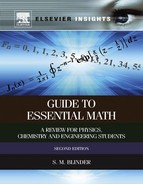
An arithmetic progression is a sequence such as 1, 4, 7, 10, 13, 16. As shown in Section 1.2, the sum of an arithmetic progression with ![]() terms is given by
terms is given by
 (7.1)
(7.1)
where ![]() is the first term,
is the first term, ![]() is the constant difference between terms, and
is the constant difference between terms, and ![]() is the last term.
is the last term.
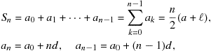
A geometric progression is a sequence which increases or decreases by a common factor ![]() , for example, 1, 3, 9, 27, 81, … or 1, 1/2, 1/4, 1/8, 1/16, … The sum of a geometric progression is given by,
, for example, 1, 3, 9, 27, 81, … or 1, 1/2, 1/4, 1/8, 1/16, … The sum of a geometric progression is given by,
 (7.2)
(7.2)
When ![]() , the sum can be carried to infinity to give
, the sum can be carried to infinity to give
![]() (7.3)
(7.3)
We had already found from the binomial theorem that
![]() (7.4)
(7.4)
By applying the binomial theorem successively to ![]() , then to each
, then to each ![]() you can show that
you can show that
 (7.5)
(7.5)
Therefore ![]() serves as a generating function for the Fibonacci numbers:
serves as a generating function for the Fibonacci numbers:
![]() (7.6)
(7.6)
An infinite geometric series inspired by one of Zeno’s paradoxes is
![]() (7.7)
(7.7)
Zeno’s paradox of motion claims that if you shoot an arrow, it can never reach its target. First it has to travel half way, then half way again—meaning 1/4 of the distance—then continue with an infinite number of steps, each taking it ![]() closer. Since infinity is so large, you’ll never get there! What we now understand that Zeno possibly didn’t (some scholars believe that his argument was meant to be satirical) was that an infinite number of decreasing terms can add up to a finite quantity.
closer. Since infinity is so large, you’ll never get there! What we now understand that Zeno possibly didn’t (some scholars believe that his argument was meant to be satirical) was that an infinite number of decreasing terms can add up to a finite quantity.
The integers 1 to to ![]() add up to
add up to
![]() (7.8)
(7.8)
while the sum of the squares is given by
![]() (7.9)
(7.9)
and the sum of the cubes by
![]() (7.10)
(7.10)
7.2 Power Series
Almost all functions can be represented by power series of the form
![]() (7.11)
(7.11)
where ![]() might be a factor such as
might be a factor such as ![]() ,
, ![]() , or
, or ![]() . The case
. The case ![]() and
and ![]() provides the most straightforward class of power series. We are already familiar with the series for the exponential function:
provides the most straightforward class of power series. We are already familiar with the series for the exponential function:
![]() (7.12)
(7.12)
as well as the sine and cosine:
![]() (7.13)
(7.13)
![]() (7.14)
(7.14)
Recall also the binomial expansion:
![]() (7.15)
(7.15)
Useful results can be obtained when power series are differentiated or integrated term by term. This is a valid procedure under very general conditions.
Consider, for example, the binomial expansion
![]() (7.16)
(7.16)
Making use of the known integral
![]() (7.17)
(7.17)
we obtain a series for the arctangent
![]() (7.18)
(7.18)
With ![]() , this gives a famous series for
, this gives a famous series for ![]()
![]() (7.19)
(7.19)
usually attributed to Gregory and Leibniz.
A second example begins with another binomial expansion
![]() (7.20)
(7.20)
We can again evaluate the integral
![]() (7.21)
(7.21)
This gives a series representation for the natural logarithm:
![]() (7.22)
(7.22)
For ![]() , this gives another famous series
, this gives another famous series
![]() (7.23)
(7.23)
As a practical matter, the convergence of this series is excruciatingly slow. It takes about 1000 terms to get ![]() correct to three significant figures,
correct to three significant figures, ![]() .
.
It is relatively simple to multiply two power series. Note that
![]() (7.24)
(7.24)
Problem 7.2.1
Evaluate the first few terms of the power series for ![]() and
and ![]() .
.
Inversion of a power series means, in principle, solving for the expansion variable ![]() as a function of the sum of the series. Consider the special case of a series in the form
as a function of the sum of the series. Consider the special case of a series in the form
![]() (7.25)
(7.25)
The constants ![]() and
and ![]() in the more general case can be absorbed into the variable
in the more general case can be absorbed into the variable ![]() and the remaining constants. Then
and the remaining constants. Then ![]() can be expanded in powers of
can be expanded in powers of ![]() in the form
in the form
![]() (7.26)
(7.26)
By a recursive procedure, carried out only as far as ![]() , we obtain:
, we obtain:
![]() (7.27)
(7.27)
Problem 7.2.2
Invert the power series for ![]() to find the first few terms in the power series for
to find the first few terms in the power series for ![]() .
.
7.3 Convergence of Series
The partial sum![]() of an infinite series is the sum of the first
of an infinite series is the sum of the first ![]() terms:
terms:
![]() (7.28)
(7.28)
The series is convergent if
![]() (7.29)
(7.29)
where ![]() is a finite quantity. A necessary condition for convergence, thus a preliminary test, is that
is a finite quantity. A necessary condition for convergence, thus a preliminary test, is that
![]() (7.30)
(7.30)
Several tests for convergence that are usually covered in introductory calculus courses. The comparison test: if a series ![]() is known to converge and
is known to converge and ![]() for all
for all ![]() , then the series
, then the series ![]() is also convergent. The ratio test: if
is also convergent. The ratio test: if ![]() then the series converges. There are more sensitive ratio tests in the case that the limit approaches 1, but you will rarely need these outside of math courses. The most useful test for convergence is the integral test. This is based on turning things around using our original definition of an integral as the limit of a sum. The sum
then the series converges. There are more sensitive ratio tests in the case that the limit approaches 1, but you will rarely need these outside of math courses. The most useful test for convergence is the integral test. This is based on turning things around using our original definition of an integral as the limit of a sum. The sum ![]() can be approximated by an integral by turning the discrete variable
can be approximated by an integral by turning the discrete variable ![]() into a continuous variable
into a continuous variable ![]() . If the integral
. If the integral
![]() (7.31)
(7.31)
is finite, then the original series converges.
A general result is that any decreasing alternating series, such as (7.23), converges. Alternating refers to the alternation of plus and minus signs. How about the analogous series with all plus signs?:
![]() (7.32)
(7.32)
After 1000 terms the sum equals 7.485. It might appear that, with sufficient patience, the series will eventually converge to a finite quantity. Not so, however! The series is divergent and sums to infinity. This can be seen by applying the integral test:
![]() (7.33)
(7.33)
A finite series of the form
![]() (7.34)
(7.34)
is called a harmonic series. Using the same approximation by an integral, we estimate that this sum is approximately equal to ![]() . The difference between
. The difference between ![]() and
and ![]() was shown by Euler to approach a constant as
was shown by Euler to approach a constant as ![]() :
:
![]() (7.35)
(7.35)
where ![]() (sometimes denoted
(sometimes denoted ![]() ) is known as the Euler-Mascheroni constant. It comes up frequently in mathematics, for example, the integral
) is known as the Euler-Mascheroni constant. It comes up frequently in mathematics, for example, the integral
![]() (7.36)
(7.36)
An alternating series is said to be absolutely convergent if the corresponding sum of absolute values, ![]() , is also convergent. This is not true for the alternating harmonic series (7.23). Such a series is said to be conditionally convergent. Conditionally convergent series must be treated with extreme caution. A theorem due to Riemann states that, by a suitable rearrangement of terms, a conditionally convergent series may be made to equal any desired value, or to diverge. Consider, for example, the series (7.20) for
, is also convergent. This is not true for the alternating harmonic series (7.23). Such a series is said to be conditionally convergent. Conditionally convergent series must be treated with extreme caution. A theorem due to Riemann states that, by a suitable rearrangement of terms, a conditionally convergent series may be made to equal any desired value, or to diverge. Consider, for example, the series (7.20) for ![]() when
when ![]() :
:
![]() (7.37)
(7.37)
Different ways of grouping the terms of the series give different answers. Thus ![]() , while
, while ![]() . But
. But ![]() actually equals 1/2. Be very careful!
actually equals 1/2. Be very careful!
7.4 Taylor Series
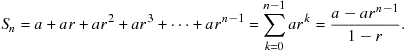
There is a systematic procedure for deriving power-series expansions for all well-behaved functions. Assuming that a function ![]() can be represented in a power series about
can be represented in a power series about ![]() , we write
, we write
![]() (7.38)
(7.38)
Clearly, when ![]() ,
,
![]() (7.39)
(7.39)
The first derivative of ![]() is given by
is given by
![]() (7.40)
(7.40)
and, setting ![]() , we obtain
, we obtain
![]() (7.41)
(7.41)
The second derivative is given by
![]() (7.42)
(7.42)
with
![]() (7.43)
(7.43)
With repeated differentiation, we find
![]() (7.44)
(7.44)
where
![]() (7.45)
(7.45)
We have therefore determined the coefficients ![]() in terms of derivatives of
in terms of derivatives of ![]() evaluated at
evaluated at ![]() and the expansion (7.38) can be given more explicitly by
and the expansion (7.38) can be given more explicitly by
 (7.46)
If the expansion is carried out around ![]() , rather than 0, the result generalizes to
, rather than 0, the result generalizes to
 (7.47)
This result is known as Taylor’s theorem and the expansion is a Taylor series. The case ![]() , given by Eq. (7.46), is sometimes called a Maclaurin series.
, given by Eq. (7.46), is sometimes called a Maclaurin series.
In order for a Taylor series around ![]() to be valid it is necessary for all derivatives
to be valid it is necessary for all derivatives ![]() to exist. The function is then said to be analytic at
to exist. The function is then said to be analytic at ![]() . A function which is not analytic at one point can still be analytic at other points. For example,
. A function which is not analytic at one point can still be analytic at other points. For example, ![]() is not analytic at
is not analytic at ![]() but is at
but is at ![]() . The series (7.22) is equivalent to an expansion of
. The series (7.22) is equivalent to an expansion of ![]() around
around ![]() .
.
We can now systematically derive all the series we obtained previously by various other methods. For example, given ![]() , we find
, we find
![]() (7.48)
(7.48)
so that (7.47) gives
![]() (7.49)
(7.49)
which is the binomial expansion. This result is seen to be valid even for noninteger values of ![]() . In the latter case we should express (7.49) in terms of the gamma function as follows:
. In the latter case we should express (7.49) in terms of the gamma function as follows:
![]() (7.50)
(7.50)
The series for ![]() is easy to derive because
is easy to derive because ![]() for all
for all ![]() . Therefore, as we have already found
. Therefore, as we have already found
![]() (7.51)
(7.51)
The Taylor series for ![]() is also straightforward since successive derivatives cycle among
is also straightforward since successive derivatives cycle among ![]() ,
, ![]() ,
, ![]() , and
, and ![]() . Since
. Since ![]() and
and ![]() , the series expansion contains only odd powers of
, the series expansion contains only odd powers of ![]() with alternating signs:
with alternating signs:
![]() (7.52)
(7.52)
Analogously, the expansion for the cosine is given by
![]() (7.53)
(7.53)
Euler’s theorem ![]() can then be deduced by comparing the series for these three functions.
can then be deduced by comparing the series for these three functions.
Problem 7.4.1
Work out the Taylor series for the function ![]() about
about ![]() , up to the term in
, up to the term in ![]() . This is a little tricky since you have to evaluate limits as
. This is a little tricky since you have to evaluate limits as ![]() to determine the derivatives
to determine the derivatives ![]() .
.
7.5 Bernoulli and Euler Numbers
The answer to Problem 7.4.1 is the series
![]() (7.54)
(7.54)
This series provides a generating function for the Bernoulli numbers, ![]() , whereby
, whereby
![]() (7.55)
(7.55)
Explicitly,
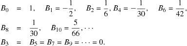 (7.56)
Bernoulli numbers find application in number theory, in numerical analysis, and in expansions of several functions related to ![]() and
and ![]() . A symbolic relation which can be used to evaluate Bernoulli numbers mimics the binomial expansion:
. A symbolic relation which can be used to evaluate Bernoulli numbers mimics the binomial expansion:
![]() (7.57)
(7.57)
where ![]() is to be replaced by
is to be replaced by ![]() .
.
We can obtain an expansion for ![]() in the following steps involving the Bernoulli numbers:
in the following steps involving the Bernoulli numbers:
![]() (7.58)
(7.58)
But
![]() (7.59)
(7.59)
Therefore
![]() (7.60)
(7.60)
and, more explicitly,
![]() (7.61)
(7.61)
Problem 7.5.1
Find the expansions for ![]() and for
and for ![]() .
.
Problem 7.5.2
From the trigonometric identity ![]() , work out the expansions for
, work out the expansions for ![]() .
.
Somewhat analogous to the definition of Bernoulli numbers are the Euler numbers![]() . These can be obtained from the generating function:
. These can be obtained from the generating function:
![]() (7.62)
(7.62)
The first few Euler numbers are
![]() (7.63)
(7.63)
with all equal to 0 for odd indices ![]() . We find directly that
. We find directly that
![]() (7.64)
(7.64)
and thus obtain the expansion
![]() (7.65)
(7.65)
Problem 7.5.3
Find the corresponding expansion for ![]() .
.
The Euler-Maclaurin sum formula provides a powerful method for evaluating some difficult summations. It actually represents a more precise connection between Riemann sums and their corresponding integrals. It can be used to approximate finite sums and even infinite series using integrals with some additional terms involving Bernoulli numbers. It can be shown that
![]() (7.66)
(7.66)
Problem 7.5.4
Using the Euler-Maclaurin formula, evaluate the sum ![]() .
.
7.6 L’Hôpital’s Rule
The value of a function is called an indeterminate form at some point ![]() if its limit as
if its limit as ![]() apparently approaches one of the forms
apparently approaches one of the forms ![]() , or
, or ![]() . Two examples are the combinations
. Two examples are the combinations ![]() and
and ![]() as
as ![]() . (As we used to say in high school, such sick functions had to be sent to L’Hôspital to be cured.) To be specific, let us consider a case for which
. (As we used to say in high school, such sick functions had to be sent to L’Hôspital to be cured.) To be specific, let us consider a case for which
![]() (7.67)
(7.67)
If ![]() and
and ![]() are both expressed in Taylor series about
are both expressed in Taylor series about ![]() ,
,
![]() (7.68)
(7.68)
If ![]() and
and ![]() both equal 0 but
both equal 0 but ![]() and
and ![]() are finite, the limit in (7.67) is given by
are finite, the limit in (7.67) is given by
![]() (7.69)
(7.69)
a result known as L’Hôpital’s rule. In the event that one or both first derivatives also vanishes, the lowest order nonvanishing derivatives in the numerator and denominator determine the limit.
To evaluate the limit of ![]() , let
, let ![]() and
and ![]() . In this case,
. In this case, ![]() . But
. But ![]() , so
, so ![]() . Also,
. Also, ![]() , for all
, for all ![]() . Therefore
. Therefore
![]() (7.70)
(7.70)
This is also consistent with the approximation that ![]() for
for ![]() . For the limit of
. For the limit of ![]() , let
, let ![]() ,
, ![]() . Now
. Now ![]() and
and ![]() . We find therefore that
. We find therefore that
![]() (7.71)
(7.71)
Problem 7.6.1
Evaluate the limit
![]()
7.7 Fourier Series
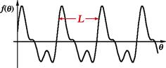
Taylor series expansions, as described above, provide a very general method for representing a large class of mathematical functions. For the special case of periodic functions, a powerful alternative method is expansion in an infinite sum of sines and cosines, known as a trigonometric series or Fourier series. A periodic function is one which repeats in value when its argument is increased by multiples of a constant ![]() , called the period or wavelength. For example,
, called the period or wavelength. For example,
![]() (7.72)
(7.72)
as shown in Figure 7.1. For convenience, let us consider the case ![]() . Sine and cosine are definitive examples of functions periodic in
. Sine and cosine are definitive examples of functions periodic in ![]() since
since
![]() (7.73)
(7.73)
The functions ![]() and
and ![]() , with
, with ![]() =integer, are also periodic in
=integer, are also periodic in ![]() (as well as in
(as well as in ![]() ).
).
A function ![]() periodic in
periodic in ![]() can be expanded as follows:
can be expanded as follows:
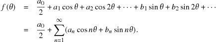 (7.74)
Writing the constant term as ![]() is convenient, as will be seen shortly. The coefficients
is convenient, as will be seen shortly. The coefficients ![]() can be determined by making use of the following definite integrals:
can be determined by making use of the following definite integrals:
![]() (7.75)
(7.75)
![]() (7.76)
(7.76)
![]() (7.77)
(7.77)
These integrals are expressed compactly with use of the Kronecker delta, defined as follows:
![]() (7.78)
(7.78)
Two functions are said to be orthogonal if the definite integral of their product equals zero. (Analogously, two vectors ![]() and
and ![]() whose scalar product
whose scalar product ![]() equals zero are said to be orthogonal—meaning perpendicular, in that context.) The set of functions
equals zero are said to be orthogonal—meaning perpendicular, in that context.) The set of functions ![]() is termed an orthogonal set in an interval of width
is termed an orthogonal set in an interval of width ![]() .
.
The nonvanishing integrals in (7.75) and (7.76) follow easily from the fact that ![]() and
and ![]() have average values of
have average values of ![]() over an integral number of wavelengths. Thus
over an integral number of wavelengths. Thus
![]() (7.79)
(7.79)
The orthogonality relations (7.75)–(7.77) enable us to determine the Fourier expansion coefficients ![]() and
and ![]() . Consider the integral
. Consider the integral ![]() , with
, with ![]() expanded using (7.74). By virtue of the orthogonality relations, only one term in the expansion survives integration:
expanded using (7.74). By virtue of the orthogonality relations, only one term in the expansion survives integration:
![]() (7.80)
(7.80)
Solving for ![]() we find
we find
![]() (7.81)
(7.81)
Note that the case ![]() correctly determines
correctly determines ![]() , by virtue of the factor
, by virtue of the factor ![]() in Eq. (7.74). Analogously, the coefficients
in Eq. (7.74). Analogously, the coefficients ![]() are given by
are given by
![]() (7.82)
(7.82)
In about half of textbooks, the limits of integration in Eqs. (7.81) and (7.82) are chosen as ![]() rather than
rather than ![]() . This is just another way to specify one period of the function and the same results are obtained in either case.
. This is just another way to specify one period of the function and the same results are obtained in either case.
As an illustration, let us calculate the Fourier expansion for a square wave, defined as follows:
![]() (7.83)
(7.83)
A square-wave oscillator is often used to test the frequency response of an electronic circuit. The Fourier coefficients can be computed using (7.81) and (7.82). First we find
![]() (7.84)
(7.84)
Thus all the cosine contributions equal zero since ![]() is symmetrical about
is symmetrical about ![]() . The square wave is evidently a Fourier sine series, with only nonvanishing
. The square wave is evidently a Fourier sine series, with only nonvanishing ![]() coefficients. We find
coefficients. We find
![]() (7.85)
(7.85)
giving
![]() (7.86)
(7.86)
The Fourier expansion for a square wave can thus be written
 (7.87)
For ![]() , Eq. (7.87) reduces to (7.19), the Gregory-Leibniz series for
, Eq. (7.87) reduces to (7.19), the Gregory-Leibniz series for ![]() :
:
![]() (7.88)
(7.88)
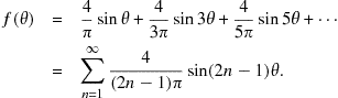
A Fourier series carried through ![]() terms is called a partial sum
terms is called a partial sum![]() . Figure 7.2 shows the function
. Figure 7.2 shows the function ![]() and the partial sums
and the partial sums ![]() , and
, and ![]() . Note how the higher partial sums overshoot near the points of discontinuity
. Note how the higher partial sums overshoot near the points of discontinuity ![]() . This is known as the Gibbs phenomenon. As
. This is known as the Gibbs phenomenon. As ![]() at these points.
at these points.

The general conditions for a periodic function ![]() to be representable by a Fourier series are the following. The function must have a finite number of maxima and minima and a finite number of discontinuities between 0 and
to be representable by a Fourier series are the following. The function must have a finite number of maxima and minima and a finite number of discontinuities between 0 and ![]() . Also,
. Also, ![]() must be finite. If these conditions are fulfilled then the Fourier series (7.74) with coefficients given by (7.81) and (7.82) converges to
must be finite. If these conditions are fulfilled then the Fourier series (7.74) with coefficients given by (7.81) and (7.82) converges to ![]() at points where the function is continuous. At discontinuities
at points where the function is continuous. At discontinuities ![]() , the Fourier series converges to the midpoint of the jump,
, the Fourier series converges to the midpoint of the jump, ![]() .
.
Recall that sines and cosines can be expressed in terms of complex exponential functions, according to Eqs. (4.60) and (4.61). Accordingly, a Fourier series can be expressed in a more compact form:
![]() (7.89)
(7.89)
where the coefficients ![]() might be complex numbers. The orthogonality relations for complex exponentials are given by
might be complex numbers. The orthogonality relations for complex exponentials are given by
![]() (7.90)
(7.90)
These determine the complex Fourier coefficients:
![]() (7.91)
(7.91)
If ![]() is a real function, then
is a real function, then ![]() for all
for all ![]() .
.
For functions with a periodicity ![]() different from
different from ![]() , the variable
, the variable ![]() can be replaced by
can be replaced by ![]() . The formulas for Fourier series are then modified as follows:
. The formulas for Fourier series are then modified as follows:
![]() (7.92)
(7.92)
with
![]() (7.93)
(7.93)
and
![]() (7.94)
(7.94)
For complex Fourier series,
![]() (7.95)
(7.95)
with
![]() (7.96)
(7.96)
Many of the applications of Fourier analysis involve the time-frequency domain. A time-dependent signal ![]() can be expressed
can be expressed
![]() (7.97)
(7.97)
where the ![]() are frequencies expressed in radians per second.
are frequencies expressed in radians per second.
When a tuning fork is struck, it emits a tone which can be represented by a sinusoidal wave—one having the shape of a sine or cosine. For tuning musical instruments, a fork might be machined to produce a pure tone at 440 Hz, which corresponds to A above middle C. (Middle C would then have a frequency of 278.4375 Hz.) The graph in Figure 7.3 shows the variation of air pressure (or density) with time for a sound wave, as measured at a single point. ![]() represents the deviation from the undisturbed atmospheric pressure
represents the deviation from the undisturbed atmospheric pressure ![]() . The maximum variation of
. The maximum variation of ![]() above or below
above or below ![]() is called the amplitude
is called the amplitude![]() of the wave. The time between successive maxima of the wave is called the period
of the wave. The time between successive maxima of the wave is called the period![]() . Since the argument of the sine or cosine varies between
. Since the argument of the sine or cosine varies between ![]() and
and ![]() in one period, the form of the wave could be the function
in one period, the form of the wave could be the function
![]() (7.98)
(7.98)
Psi (![]() ) is a very common symbol for wave amplitude. The frequency
) is a very common symbol for wave amplitude. The frequency![]() , defined by
, defined by
![]() (7.99)
(7.99)
gives the number of oscillations per second, conventionally expressed in hertz (Hz). An alternative measure of frequency is the number of radians per second, ![]() . Since one cycle corresponds to
. Since one cycle corresponds to ![]() radians,
radians,
![]() (7.100)
(7.100)
The upper strip in Figure 7.3 shows the profile of the sound wave at a single instant of time. The pressure or density of the air also has a sinusoidal shape. At some given instant of time ![]() the deviation of pressure from the undisturbed presssure
the deviation of pressure from the undisturbed presssure ![]() might be represented by
might be represented by
![]() (7.101)
(7.101)
where ![]() is the wavelength of the sound, the distance between successive pressure maxima. Sound consists of longitudinal waves, in which the wave amplitude varies in the direction parallel to the wave’s motion. By contrast, electromagnetic waves, such as light, are transverse, with their electric and magnetic fields oscillating perpendicular to the direction of motion. The speed of light in vacuum,
is the wavelength of the sound, the distance between successive pressure maxima. Sound consists of longitudinal waves, in which the wave amplitude varies in the direction parallel to the wave’s motion. By contrast, electromagnetic waves, such as light, are transverse, with their electric and magnetic fields oscillating perpendicular to the direction of motion. The speed of light in vacuum, ![]() m/s. The speed of sound in air is much slower, typically around 350 m/s (1100 ft/s or 770 miles/hr—known as Mach 1 for jet planes). As you know, thunder is the sound of lightning. You see the lightning essentially instantaneously but thunder takes about 5 s to travel 1 mile. You can calculate how far away a storm is by counting the number of seconds between the lightning and the thunder. A wave (light or sound) traveling at a speed
m/s. The speed of sound in air is much slower, typically around 350 m/s (1100 ft/s or 770 miles/hr—known as Mach 1 for jet planes). As you know, thunder is the sound of lightning. You see the lightning essentially instantaneously but thunder takes about 5 s to travel 1 mile. You can calculate how far away a storm is by counting the number of seconds between the lightning and the thunder. A wave (light or sound) traveling at a speed ![]() moves a distance of one wavelength
moves a distance of one wavelength ![]() in the time of one period
in the time of one period ![]() . This implies the general relationship between frequency and wavelength
. This implies the general relationship between frequency and wavelength
![]() (7.102)
(7.102)
valid for all types of wave phenomena. A trumpet playing the same sustained note produces a much richer sound than a tuning fork, as shown in Figure 7.4. Fourier analysis of a musical tone shows a superposition of the fundamental frequency ![]() augmented by harmonics or overtones, which are integer multiples of
augmented by harmonics or overtones, which are integer multiples of ![]() .
.


7.8 Dirac Deltafunction
Recall that the Kronecker delta ![]() , defined in Eq. (7.78), pertains to the discrete variables
, defined in Eq. (7.78), pertains to the discrete variables ![]() and
and ![]() . A useful application enables the reduction of a summation to a single term:
. A useful application enables the reduction of a summation to a single term:
![]() (7.103)
(7.103)
The analog of the Kronecker delta for continuous variables is the Dirac deltafunction![]() , which has the defining property
, which has the defining property
![]() (7.104)
(7.104)
which includes the normalization condition
![]() (7.105)
(7.105)
Evidently
![]() (7.106)
(7.106)
The approach to ![]() is sufficiently tame, however, that the integral has a finite value.
is sufficiently tame, however, that the integral has a finite value.
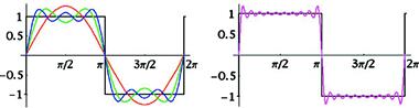
A simple representation for the deltafunction is the limit of a normalized Gaussian as the standard deviation approaches zero:
![]() (7.107)
(7.107)
The Dirac deltafunction is shown pictorially in Figure 7.5. The deltafunction is the limit of a function which becomes larger and larger in an interval which becomes narrower and narrower. (Some university educators bemoaning increased specialization contend that graduate students are learning more and more about less and less until they eventually wind up knowing everything about nothing—the ultimate deltafunction!)
Differentiation of a function at a finite discontinuity produces a deltafunction. Consider, for example, the Heaviside unit step function:
![]() (7.108)
(7.108)
Sometimes ![]() (for
(for ![]() ) is defined as
) is defined as ![]() . The derivative of the Heaviside function
. The derivative of the Heaviside function ![]() is clearly equal to zero when
is clearly equal to zero when ![]() . In addition
. In addition
![]() (7.109)
(7.109)
We can thus identify
![]() (7.110)
(7.110)
The deltafunction can be generalized to multiple dimensions. In three dimensions, the defining relation for a deltafunction can be expressed
![]() (7.111)
(7.111)
For example, the limit of a continuous distribution of electrical charge ![]() shrunken to a point charge
shrunken to a point charge ![]() at
at ![]() can be represented by
can be represented by
![]() (7.112)
(7.112)
The potential energy of interaction between two continuous charge distributions is given by
![]() (7.113)
(7.113)
If the distribution ![]() is reduced to a point charge
is reduced to a point charge ![]() at
at ![]() , this reduces to
, this reduces to
![]() (7.114)
(7.114)
If the analogous thing then happens to ![]() , the formula reduces to the Coulomb potential energy between two point charges
, the formula reduces to the Coulomb potential energy between two point charges
![]() (7.115)
(7.115)
Problem 7.8.1
Show that the normalized Lorentzian distribution
![]()
approaches a deltafunction in the limit as ![]() .
.
7.9 Fourier Integrals
Fourier series are ideal for periodic functions, sums over frequencies which are integral multiples of some ![]() . For a more general class of functions which are not simply periodic, all possible frequency contributions must be considered. This can be accomplished by replacing a discrete Fourier series by a continuous integral. The coefficients
. For a more general class of functions which are not simply periodic, all possible frequency contributions must be considered. This can be accomplished by replacing a discrete Fourier series by a continuous integral. The coefficients ![]() (or, equivalently,
(or, equivalently, ![]() and
and ![]() ) which represent the relative weight of each harmonic will turn into a Fourier transform
) which represent the relative weight of each harmonic will turn into a Fourier transform![]() , which measures the contribution of a frequency in a continuous range of
, which measures the contribution of a frequency in a continuous range of ![]() . In the limit as
. In the limit as ![]() , a complex Fourier series (7.95) generalizes to a Fourier integral. The discrete variable
, a complex Fourier series (7.95) generalizes to a Fourier integral. The discrete variable ![]() can be replaced by a continuous variable
can be replaced by a continuous variable ![]() , such that
, such that
![]() (7.116)
(7.116)
with the substitution
![]() (7.117)
(7.117)
Correspondingly, Eq. (7.96) becomes
![]() (7.118)
(7.118)
where ![]() is called the Fourier transform of
is called the Fourier transform of ![]() —alternatively written
—alternatively written ![]() ,
, ![]() ,
, ![]() ,
, ![]() or sometimes simply
or sometimes simply ![]() . A Fourier-transform pair
. A Fourier-transform pair ![]() and
and ![]() can also be defined more symmetrically by writing:
can also be defined more symmetrically by writing:
![]() (7.119)
(7.119)
Fourier integrals in the time-frequency domain have the form
![]() (7.120)
(7.120)
Figure 7.4 is best described as a Fourier transform of a trumpet tone since the spectrum of frequencies consists of peaks of finite width.
Another representation of the deltafunction, useful in the manipulation of Fourier transforms, is defined by the limit:
![]() (7.121)
(7.121)
For ![]() , the function equals
, the function equals ![]() , which approaches
, which approaches ![]() . For
. For ![]() the sine function oscillates with ever-increasing frequency as
the sine function oscillates with ever-increasing frequency as ![]() . The positive and negative contributions cancel so that the function becomes essentially equivalent to 0 under the integral sign. Finally, since
. The positive and negative contributions cancel so that the function becomes essentially equivalent to 0 under the integral sign. Finally, since
![]() (7.122)
(7.122)
for finite values of k, Eq. (7.121) is suitably normalized to represent a deltafunction. The significance of this last representation is shown by the integral
 (7.123)
This shows that the Fourier transform of a complex monochromatic wave ![]() is a deltafunction
is a deltafunction ![]() .
.
An important result for Fourier transforms can be derived using (7.123). Using the symmetrical form for the Fourier integral (7.119), we can write
 (7.124)
being careful to use the dummy variable ![]() in the second integral on the right. The integral over
in the second integral on the right. The integral over ![]() on the right then gives
on the right then gives
![]() (7.125)
(7.125)
Following this by integration over ![]() we obtain
we obtain
![]() (7.126)
(7.126)
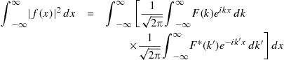
a result known as Parseval’s theorem. A closely related result is Plancherel’s theorem:
![]() (7.127)
(7.127)
where ![]() and
and ![]() are the symmetric Fourier transforms of
are the symmetric Fourier transforms of ![]() and
and ![]() , respectively.
, respectively.
The convolution of two functions is defined by
![]() (7.128)
(7.128)
The Fourier transform of a convolution integral can be found by substituting the symmetric Fourier transforms ![]() and
and ![]() and using the deltafunction formula (7.125). The result is the convolution theorem, which can be expressed very compactly as
and using the deltafunction formula (7.125). The result is the convolution theorem, which can be expressed very compactly as
![]() (7.129)
(7.129)
In an alternative form, ![]() .
.
7.10 Generalized Fourier Expansions
For Bessel functions and other types of special functions to be introduced later, it is possible to construct orthonormal sets of basis functions ![]() which satisfy the orthogonality and normalization conditions:
which satisfy the orthogonality and normalization conditions:
![]() (7.130)
(7.130)
with respect to integration over appropriate limits. (If the functions are real, complex conjugation is unnecessary.) An arbitrary function ![]() in the same domain as the basis functions can be expanded in an expansion analogous to a Fourier series
in the same domain as the basis functions can be expanded in an expansion analogous to a Fourier series
![]() (7.131)
(7.131)
with the coefficients determined by
![]() (7.132)
(7.132)
If (7.132) is substituted into (7.131), with the appropriate use of a dummy variable, we obtain
![]() (7.133)
(7.133)
The last quantity in square brackets has the same effect as the deltafunction ![]() . The relation known as closure
. The relation known as closure
![]() (7.134)
(7.134)
is, in a sense, complementary to the orthonormality condition (7.130).
Generalized Fourier series find extensive application in mathematical physics, particularly quantum mechanics.
7.11 Asymptotic Series
In certain circumstances, a divergent series can be used to determine approximate values of a function as ![]() . Consider, as an example, the complementary error function
. Consider, as an example, the complementary error function ![]() , defined in Eq. (6.95):
, defined in Eq. (6.95):
![]() (7.135)
(7.135)
Noting that
![]() (7.136)
(7.136)
Equation (7.135) can be integrated by parts to give
![]() (7.137)
(7.137)
Integrating by parts again:
![]() (7.138)
(7.138)
Continuing the process, we obtain
![]() (7.139)
(7.139)
This is an instance of an asymptotic series, as indicated by the equivalence symbol ![]() rather than an equal sign. The series in brackets is actually divergent. However, a finite number of terms gives an approximation to
rather than an equal sign. The series in brackets is actually divergent. However, a finite number of terms gives an approximation to ![]() for large values of
for large values of ![]() . The omitted terms, when expressed in their original form as an integral, as in Eqs. (7.137) or (7.138), approach zero as
. The omitted terms, when expressed in their original form as an integral, as in Eqs. (7.137) or (7.138), approach zero as ![]() .
.
Consider the general case of an asymptotic series
![]() (7.140)
(7.140)
with a partial sum
![]() (7.141)
(7.141)
The condition for ![]() to be an asymptotic representation for
to be an asymptotic representation for ![]() can be expressed
can be expressed
![]() (7.142)
(7.142)
A convergent series approaches ![]() for a given
for a given ![]() as
as ![]() , where
, where ![]() is the number of terms in the partial sum
is the number of terms in the partial sum ![]() . By contrast, an asymptotic series approaches
. By contrast, an asymptotic series approaches ![]() as
as ![]() for a given
for a given ![]() .
.
The exponential integral is another function defined as a definite integral which cannot be evaluated in a simple closed form. In the usual notation
![]() (7.143)
(7.143)
By repeated integration by parts, the following asymptotic series for the exponential integral can be derived:
![]() (7.144)
(7.144)
Finally, we will derive an asymptotic expansion for the gamma function, applying a technique known as the method of steepest descents. Recall the integral definition:
![]() (7.145)
(7.145)
For large ![]() the integrand
the integrand ![]() will be very sharply peaked around
will be very sharply peaked around ![]() . It is convenient to write
. It is convenient to write
![]() (7.146)
(7.146)
A Taylor series expansion of ![]() about
about ![]() gives
gives
 (7.147)
noting that ![]() . The integral (7.145) can then be approximated as follows:
. The integral (7.145) can then be approximated as follows:
![]() (7.148)
(7.148)
For large ![]() , we introduce a negligible error by extending the lower integration limit to
, we introduce a negligible error by extending the lower integration limit to ![]() . The integral can then be done exactly to give Stirling’s formula
. The integral can then be done exactly to give Stirling’s formula
![]() (7.149)
(7.149)
or in terms of the factorial
![]() (7.150)
(7.150)
This is consistent with the well-known approximation for the natural logarithm:
![]() (7.151)
(7.151)
A more complete asymptotic expansion for the gamma function will have the form
![]() (7.152)
(7.152)
Making use of the recursion relation
![]() (7.153)
(7.153)
it can be shown that ![]() and
and ![]() .
.
You will notice that, as we go along, we are leaving more and more computational details for you to work out on your own. Hopefully, your mathematical facility is improving at a sufficient rate to keep everything understandable.