
Complex Variables
A deeper understanding of functional analysis, even principles involving real functions of real variables, can be attained if the functions and variables are extended into the complex plane. Figure 14.1 shows schematically how a functional relationship ![]() can be represented by a mapping of the z-plane, with
can be represented by a mapping of the z-plane, with ![]() , into the w-plane, with
, into the w-plane, with ![]() .
.
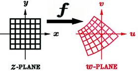
Figure 14.1 Mapping of the functional relation ![]() . If the function is analytic, then the mapping is conformal, with orthogonality of grid lines preserved.
. If the function is analytic, then the mapping is conformal, with orthogonality of grid lines preserved.
14.1 Analytic Functions
Let
![]() (14.1)
(14.1)
be a complex-valued function constructed from two real functions ![]() and
and ![]() . Under what conditions can
. Under what conditions can ![]() be considered a legitimate function of a single complex variable
be considered a legitimate function of a single complex variable ![]() , allowing us to write
, allowing us to write ![]() ? A simple example would be
? A simple example would be
![]() (14.2)
(14.2)
so that
![]() (14.3)
(14.3)
Evidently
![]() (14.4)
(14.4)
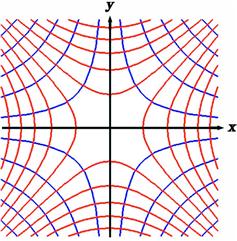
This function can be represented in the complex plane as shown in Figure 14.2. A counterexample, which is not a legitimate function of a complex variable, would be
![]() (14.5)
(14.5)
since the complex conjugate ![]() is not considered a function of z. To derive a general condition for
is not considered a function of z. To derive a general condition for ![]() , express x and y in terms of z and
, express x and y in terms of z and ![]() using
using
![]() (14.6)
(14.6)
An arbitrary function in Eq. (14.1) can thus be reexpressed in the functional form ![]() . The condition that
. The condition that ![]() , with no dependence on
, with no dependence on ![]() , implies that
, implies that
![]() (14.7)
(14.7)
We can write
![]() (14.8)
(14.8)
Using (14.6), this reduces to
![]() (14.9)
(14.9)
Since the real and imaginary parts must individually equal zero, we obtain the Cauchy-Riemann equations:
![]() (14.10)
(14.10)
These conditions on the real and imaginary parts of a function ![]() must be fulfilled in order for w to a function of the complex variable z. If, in addition, u and
must be fulfilled in order for w to a function of the complex variable z. If, in addition, u and ![]() have continuous partial derivatives with respect to x and y in some region, then
have continuous partial derivatives with respect to x and y in some region, then ![]() in that region is an analytic function of z. In complex analysis, the term holomorphic function is often used to distinguish it from a real analytic function.
in that region is an analytic function of z. In complex analysis, the term holomorphic function is often used to distinguish it from a real analytic function.
A complex variable z can alternatively be expressed in polar form
![]() (14.11)
(14.11)
where ![]() is referred to as the modulus and
is referred to as the modulus and ![]() , the phase or argument. Correspondingly, the function
, the phase or argument. Correspondingly, the function ![]() would be written
would be written
![]() (14.12)
(14.12)
The Cauchy-Riemann equations in polar form are then given by
![]() (14.13)
(14.13)
Consider the function
![]() (14.14)
(14.14)
Both ![]() and
and ![]() and their x- and y-derivatives are well behaved everywhere in the
and their x- and y-derivatives are well behaved everywhere in the ![]() -plane except at the point
-plane except at the point ![]() , where they become discontinuous and, in fact, infinite. In mathematical jargon, the function and its derivatives do not exist at that point. We say therefore that
, where they become discontinuous and, in fact, infinite. In mathematical jargon, the function and its derivatives do not exist at that point. We say therefore that ![]() is an analytic function in the entire complex plane except at the point
is an analytic function in the entire complex plane except at the point ![]() . A value of z at which a function is not analytic is called a singular point or singularity.
. A value of z at which a function is not analytic is called a singular point or singularity.
Taking the x-derivative of the first Cauchy-Riemann equation and the y-derivative of the second, we have
![]() (14.15)
(14.15)
Since the mixed second derivatives of ![]() are equal,
are equal,
![]() (14.16)
(14.16)
Analogously, we find
![]() (14.17)
(14.17)
Therefore both the real and imaginary parts of an analytic function are solution of the two-dimensional Laplace equation, known as harmonic functions. This can be verified for ![]() and
and ![]() , given in the above example of the analytic function
, given in the above example of the analytic function ![]() .
.
14.2 Derivative of an Analytic Function
The derivative of a complex function is given by the obvious transcription of the definition used for real functions:
![]() (14.18)
(14.18)
In the definition of a real derivative, such as ![]() or
or ![]() , there is only one way for
, there is only one way for ![]() or
or ![]() to approach zero. For
to approach zero. For ![]() in the complex plane, there are however an infinite number of ways to approach
in the complex plane, there are however an infinite number of ways to approach ![]() . For an analytic function, all of them should give the same result for the derivative.
. For an analytic function, all of them should give the same result for the derivative.
Let us consider two alternative ways to achieve the limit ![]() : (1) along the x-axis with
: (1) along the x-axis with ![]() or (2) along the y-axis with
or (2) along the y-axis with ![]() . With
. With ![]() , we can write
, we can write
![]() (14.19)
(14.19)
with
![]() (14.20)
(14.20)
The limits for ![]() in the alternative processes are then given by
in the alternative processes are then given by
![]() (14.21)
(14.21)
and
![]() (14.22)
(14.22)
Equating the real and imaginary parts of (14.21) and (14.22), we again arrive at the Cauchy-Riemann Eqs. (14.10).
All the familiar formulas for derivatives remain valid for complex variables, for example, ![]() , and so forth.
, and so forth.
14.3 Contour Integrals
The integral of a complex function ![]() has the form of a line integral (see Section 11.7) over a specified path or contour C between two points
has the form of a line integral (see Section 11.7) over a specified path or contour C between two points ![]() and
and ![]() in the complex plane. It is defined as the analogous limit of a Riemann sum:
in the complex plane. It is defined as the analogous limit of a Riemann sum:
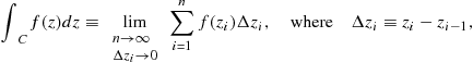 (14.23)
where the points ![]() lie on a continuous path C between
lie on a continuous path C between ![]() and
and ![]() . In the most general case, the value of the integral depends on the path C. For the case of an analytic function in a simply connected region, we will show that the contour integral is independent of path, being determined entirely by the endpoints
. In the most general case, the value of the integral depends on the path C. For the case of an analytic function in a simply connected region, we will show that the contour integral is independent of path, being determined entirely by the endpoints ![]() and
and ![]() .
.
14.4 Cauchy’s Theorem
This is the central result in the theory of complex variables. It states that the line integral of an analytic function around an arbitrary closed path in a simple-connected region vanishes:
![]() (14.24)
(14.24)
The path of integration is understood to be traversed in the counterclockwise sense. An “informal” proof can be based on the identification of ![]() with an exact differential expression (see Section 11.6):
with an exact differential expression (see Section 11.6):
![]() (14.25)
(14.25)
It is seen that Euler’s reciprocity relation (11.48)
![]() (14.26)
(14.26)
is equivalent to the Cauchy-Riemann Eqs. (14.10). Cauchy’s theorem is then a simple transcription of the result (11.73) for the line integral around a closed path. The region in play must be simply connected, with no singularities. Equation (14.24) is sometimes referred to as the Cauchy-Goursat theorem. Goursat proved it under somewhat less restrictive conditions, showing that ![]() need not be a continuous function.
need not be a continuous function.
14.5 Cauchy’s Integral Formula
The most important applications of Cauchy’s theorem involve functions with singular points. Consider the integral
![]()
around the closed path C shown in Figure 14.3. Let ![]() be an analytic function in the entire region. Then
be an analytic function in the entire region. Then ![]() is also analytic except at the point
is also analytic except at the point ![]() . The contour C can be shrunken to a small circle
. The contour C can be shrunken to a small circle ![]() surrounding
surrounding ![]() , as shown in the figure. The infinitesimally narrow channel connecting C to
, as shown in the figure. The infinitesimally narrow channel connecting C to ![]() is traversed in both directions, thus canceling its contribution to the integral around the composite contour. By Cauchy’s theorem
is traversed in both directions, thus canceling its contribution to the integral around the composite contour. By Cauchy’s theorem
![]() (14.27)
(14.27)
The minus sign appears because the integration is clockwise around the circle ![]() . We find therefore
. We find therefore
![]() (14.28)
(14.28)
assuming that ![]() is a sufficiently small circle that
is a sufficiently small circle that ![]() is nearly constant within, well approximated as
is nearly constant within, well approximated as ![]() . It is convenient now to switch to a polar representation of the complex variable, with
. It is convenient now to switch to a polar representation of the complex variable, with
![]() (14.29)
(14.29)
We find then
![]() (14.30)
(14.30)
The result is Cauchy’s integral theorem:
![]() (14.31)
(14.31)
A remarkable implication of this formula is a sort of holographic principle. If the values of an analytic function ![]() are known on the boundary of a region, then the value of the function can be determined at every point
are known on the boundary of a region, then the value of the function can be determined at every point ![]() inside that region.
inside that region.

Cauchy’s integral formula can be differentiated with respect to ![]() any number of times to give
any number of times to give
![]() (14.32)
(14.32)
and, more generally,
![]() (14.33)
(14.33)
This shows, incidentally, that derivatives of all orders exist for an analytic function.
14.6 Taylor Series
Taylor’s theorem can be derived from the Cauchy integral theorem. Let us first rewrite (14.31) as
![]() (14.34)
(14.34)
where ![]() is now the variable of integration along the contour C and z, any point in the interior of the contour. Let us develop a power-series expansion of
is now the variable of integration along the contour C and z, any point in the interior of the contour. Let us develop a power-series expansion of ![]() around the point
around the point ![]() , also within the contour. Applying the binomial theorem, we can write
, also within the contour. Applying the binomial theorem, we can write
![]() (14.35)
(14.35)
Note that ![]() so that
so that ![]() and the series converges. Substituting the summation into (14.34), we obtain
and the series converges. Substituting the summation into (14.34), we obtain
![]() (14.36)
(14.36)
Therefore, using Cauchy’s integral theorem (14.33),
![]() (14.37)
(14.37)
This shows that a function analytic in a region can be expanded in a Taylor series about a point ![]() within that region. The series (14.37) will converge to
within that region. The series (14.37) will converge to ![]() within a certain radius of convergence, a circle of radius
within a certain radius of convergence, a circle of radius ![]() , equal to the distance to
, equal to the distance to ![]() , the singular point closest to
, the singular point closest to ![]() .
.
We can now understand the puzzling behavior of the series
![]() (14.38)
(14.38)
which we encountered in Eq. (7.37). The complex function ![]() has a singularity at
has a singularity at ![]() . Thus an expansion about
. Thus an expansion about ![]() will be valid only within a circle of radius of 1 around the origin. This means that a Taylor series about
will be valid only within a circle of radius of 1 around the origin. This means that a Taylor series about ![]() will be valid only for
will be valid only for ![]() . On the real axis this corresponds to
. On the real axis this corresponds to ![]() and means that both the series
and means that both the series ![]() and
and ![]() will converge only under this condition. The function
will converge only under this condition. The function ![]() could, however, be expanded about
could, however, be expanded about ![]() , giving a larger radius of convergence
, giving a larger radius of convergence ![]() . Along the real axis, we find
. Along the real axis, we find
![]() (14.39)
(14.39)
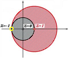
The process of shifting the domain of a Taylor series is known as analytic continuation. Figure 14.4 shows the circles of convergence for ![]() expanded about
expanded about ![]() and about
and about ![]() . Successive applications of analytic continuation can cover the entire complex plane, exclusive of singular points (with some limitations for multivalued functions).
. Successive applications of analytic continuation can cover the entire complex plane, exclusive of singular points (with some limitations for multivalued functions).
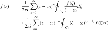
14.7 Laurent Expansions
Taylor series are valid expansions of ![]() about points
about points ![]() (sometimes called regular points) within the region where the function is analytic. It is also possible to expand a function about singular points. Figure 14.5 outlines an annular (shaped like a lock washer) region around a singularity
(sometimes called regular points) within the region where the function is analytic. It is also possible to expand a function about singular points. Figure 14.5 outlines an annular (shaped like a lock washer) region around a singularity ![]() of a function
of a function ![]() , but avoiding other singularities at
, but avoiding other singularities at ![]() and
and ![]() . The function is integrated around the contour including
. The function is integrated around the contour including ![]() in a counterclockwise sense,
in a counterclockwise sense, ![]() in a clockwise sense, and the connecting cut in canceling directions. Denoting the complex variable on the contour by
in a clockwise sense, and the connecting cut in canceling directions. Denoting the complex variable on the contour by ![]() , we can apply Cauchy’s theorem to obtain
, we can apply Cauchy’s theorem to obtain
![]() (14.40)
(14.40)
where z is any point within the annular region. On the contour ![]() we have
we have ![]() so that
so that ![]() , validating the convergent expansion (14.35):
, validating the convergent expansion (14.35):
![]() (14.41)
(14.41)
On the contour ![]() , however,
, however, ![]() so that
so that ![]() and we have instead
and we have instead
![]() (14.42)
(14.42)
where we have inverted the fractions in the last summation and shifted the dummy index. Substituting the last two expansions into (14.40), we obtain
 (14.43)
This is a summation containing both positive and negative powers of ![]() :
:
![]() (14.44)
(14.44)
known as a Laurent series. The coefficients are given by
![]() (14.45)
(14.45)
where C is any counterclockwise contour within the annular region encircling the point ![]() . The result can also be combined into a single summation
. The result can also be combined into a single summation
![]() (14.46)
(14.46)
with ![]() now understood to be defined for both positive and negative n.
now understood to be defined for both positive and negative n.

Figure 14.5 Contour for derivation of Laurent expansion of ![]() about singular point
about singular point ![]() . The singularities at
. The singularities at ![]() and
and ![]() are avoided.
are avoided.
When ![]() for all n, the Laurent expansion reduces to an ordinary Taylor series. A function with some negative power of
for all n, the Laurent expansion reduces to an ordinary Taylor series. A function with some negative power of ![]() in its Laurent expansion has, of necessity, a singularity at
in its Laurent expansion has, of necessity, a singularity at ![]() . If the lowest negative power is
. If the lowest negative power is ![]() (with
(with ![]() for
for ![]() ), then
), then ![]() is said to have a pole of order N at
is said to have a pole of order N at ![]() . If
. If ![]() , so that
, so that ![]() is the lowest-power contribution, then
is the lowest-power contribution, then ![]() is called a simple pole. For example,
is called a simple pole. For example, ![]() has a simple pole at
has a simple pole at ![]() and a pole of order 2 at
and a pole of order 2 at ![]() . If the Laurent series does not terminate, the function is said to have an essential singularity. For example, the exponential of a reciprocal,
. If the Laurent series does not terminate, the function is said to have an essential singularity. For example, the exponential of a reciprocal,
![]() (14.47)
(14.47)
has an essential singularity at ![]() . The poles in a Laurent expansion are instances of isolated singularities, to be distinguished from continuous arrays of singularities which can also occur.
. The poles in a Laurent expansion are instances of isolated singularities, to be distinguished from continuous arrays of singularities which can also occur.
14.8 Calculus of Residues
In a Laurent expansion for ![]() within the region enclosed by C, the coefficient
within the region enclosed by C, the coefficient ![]() (or
(or ![]() ) of the term
) of the term ![]() is given by
is given by
![]() (14.48)
(14.48)
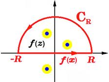
This is called the residue of ![]() and plays a very significant role in complex analysis. If a function contains several singular points within the contour C, the contour can be shrunken to a series of small circles around the singularities
and plays a very significant role in complex analysis. If a function contains several singular points within the contour C, the contour can be shrunken to a series of small circles around the singularities ![]() , as shown in Figure 14.6. The residue theorem states that the value of the contour integral is given by
, as shown in Figure 14.6. The residue theorem states that the value of the contour integral is given by
![]() (14.49)
(14.49)
If a function ![]() , as represented by a Laurent series (14.44) or (14.46), is integrated term by term, the respective contributions are given by
, as represented by a Laurent series (14.44) or (14.46), is integrated term by term, the respective contributions are given by
![]() (14.50)
(14.50)
Only the contribution from ![]() will survive—hence the designation “residue.”
will survive—hence the designation “residue.”
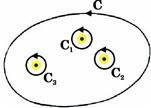
Figure 14.6 The contour for the integral ![]() can be shrunken to enclose just the singular points of
can be shrunken to enclose just the singular points of ![]() . This is applied in derivation of the theorem of residues.
. This is applied in derivation of the theorem of residues.
The residue of ![]() at a simple pole
at a simple pole ![]() is easy to find:
is easy to find:
![]() (14.51)
(14.51)
At a pole of order N, the residue is a bit more complicated:
![]() (14.52)
(14.52)
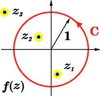
The calculus of residues can be applied to the evaluation of certain types of real integrals. Consider first a trigonometric integral of the form
![]() (14.53)
(14.53)
With a change of variables to ![]() , this can be transformed into a contour integral around the unit circle, as shown in Figure 14.7. Note that
, this can be transformed into a contour integral around the unit circle, as shown in Figure 14.7. Note that
![]() (14.54)
(14.54)
so that ![]() can be expressed as
can be expressed as ![]() . Also
. Also ![]() . Therefore the integral becomes
. Therefore the integral becomes
![]() (14.55)
(14.55)
and can be evaluated by finding all the residues of ![]() inside the unit circle:
inside the unit circle:
![]() (14.56)
(14.56)
As an example, consider the integral
![]() (14.57)
(14.57)
This is equal to the contour integral
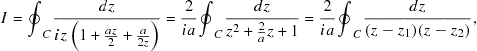 (14.58)
where
![]() (14.59)
(14.59)
The pole at ![]() lies outside the unit circle when
lies outside the unit circle when ![]() . Thus we need include only the residue of the integrand at
. Thus we need include only the residue of the integrand at ![]() :
:
![]() (14.60)
(14.60)
Finally, therefore,
![]() (14.61)
(14.61)
An infinite integral of the form
![]() (14.62)
(14.62)
can also be evaluated by the calculus of residues provided that the complex function ![]() is analytic in the upper half plane with a finite number of poles. It is also necessary for
is analytic in the upper half plane with a finite number of poles. It is also necessary for ![]() to approach zero more rapidly than
to approach zero more rapidly than ![]() as
as ![]() in the upper half plane. Consider, for example,
in the upper half plane. Consider, for example,
![]() (14.63)
(14.63)
The contour integral over a semicircular sector shown in Figure 14.8 has the value
![]() (14.64)
(14.64)
On the semicircular arc ![]() , we can write
, we can write ![]() so that
so that
![]() (14.65)
(14.65)
Thus, as ![]() , the contribution from the semicircle vanishes while the limits of the x-integral extend to
, the contribution from the semicircle vanishes while the limits of the x-integral extend to ![]() . The function
. The function ![]() has simple poles at
has simple poles at ![]() . Only the pole at
. Only the pole at ![]() is in the upper half plane, with
is in the upper half plane, with ![]() , therefore
, therefore
![]() (14.66)
(14.66)
Problem 14.8.1
Evaluate the following integrals:
![]()
14.9 Multivalued Functions
Thus far we have considered single-valued functions, which are uniquely specified by an independent variable z. The simplest counterexample is the square root ![]() which is a two-valued function. Even in the real domain,
which is a two-valued function. Even in the real domain, ![]() can equal either
can equal either ![]() . When the complex function
. When the complex function ![]() is expressed in polar form
is expressed in polar form
![]() (14.67)
(14.67)
it is seen that the full range of ![]() requires that
requires that ![]() vary from 0 to
vary from 0 to ![]() (not just
(not just ![]() ). This means that the complex z-plane must be traversed twice in order to attain all possible values of
). This means that the complex z-plane must be traversed twice in order to attain all possible values of ![]() . The extended domain of z can be represented as a Riemann surface—constructed by duplication of the complex plane, as shown in Figure 14.9. The Riemann surface corresponds to the full domain of a complex variable z. For purposes of visualization, the surface is divided into connected Riemann sheets, each of which is a conventional complex plane. Thus the Riemann surface for
. The extended domain of z can be represented as a Riemann surface—constructed by duplication of the complex plane, as shown in Figure 14.9. The Riemann surface corresponds to the full domain of a complex variable z. For purposes of visualization, the surface is divided into connected Riemann sheets, each of which is a conventional complex plane. Thus the Riemann surface for ![]() consists of two Riemann sheets connected along a branch cut, which is conveniently chosen as the negative real axis. A Riemann sheet represents a single branch of a multivalued function. For example, the first Riemann sheet of the square-root function produces values
consists of two Riemann sheets connected along a branch cut, which is conveniently chosen as the negative real axis. A Riemann sheet represents a single branch of a multivalued function. For example, the first Riemann sheet of the square-root function produces values ![]() in the range
in the range ![]() , while the second sheet is generated by
, while the second sheet is generated by ![]() . A point contained in every Riemann sheet,
. A point contained in every Riemann sheet, ![]() in the case of the square-root function, is called a branch point. The trajectory of the branch cut beginning at the branch point is determined by convenience or convention. Thus the branch cut for
in the case of the square-root function, is called a branch point. The trajectory of the branch cut beginning at the branch point is determined by convenience or convention. Thus the branch cut for ![]() could have been chosen as any path from
could have been chosen as any path from ![]() to
to ![]() .
.
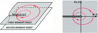
Figure 14.9 Representations of Riemann surface for ![]() . The dashed segments of the loops lie on the second Riemann sheet.
. The dashed segments of the loops lie on the second Riemann sheet.
The Riemann surface for the cube root ![]() comprises three Riemann sheets, corresponding to three branches of the function. Analogously, any integer or rational power of z will have a finite number of branches. However, an irrational power such as
comprises three Riemann sheets, corresponding to three branches of the function. Analogously, any integer or rational power of z will have a finite number of branches. However, an irrational power such as ![]() will not be periodic in any integer multiple of
will not be periodic in any integer multiple of ![]() and will hence require an infinite number of Riemann sheets. The same is true of the complex logarithmic function
and will hence require an infinite number of Riemann sheets. The same is true of the complex logarithmic function
![]() (14.68)
(14.68)
and of the inverse of any periodic function, including ![]() , etc. In such cases, the Riemann surface can be imagined as an infinite helical (or spiral) ramp, as shown in Figure 14.10.
, etc. In such cases, the Riemann surface can be imagined as an infinite helical (or spiral) ramp, as shown in Figure 14.10.
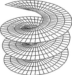
Figure 14.10 Schematic representation of several sheets of the Riemann surface needed to cover the domain of a multivalued function such as ![]() , or
, or ![]() .
.
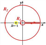
Branch cuts can be exploited in the evaluation of certain integrals, for example
![]()
with ![]() . Consider the corresponding complex integral around the contour shown in Figure 14.11. A small and a large circle of radii
. Consider the corresponding complex integral around the contour shown in Figure 14.11. A small and a large circle of radii ![]() and
and ![]() , respectively, are joined by a branch cut along the positive real axis. We can write
, respectively, are joined by a branch cut along the positive real axis. We can write
![]() (14.69)
(14.69)
Along the upper edge of the branch cut we take ![]() . Along the lower edge, however, the phase of z has increased by
. Along the lower edge, however, the phase of z has increased by ![]() , so that, in noninteger powers,
, so that, in noninteger powers, ![]() . In the limit as
. In the limit as ![]() and
and ![]() , the contributions from both circular contours approach zero. The only singular point within the contour C is at
, the contributions from both circular contours approach zero. The only singular point within the contour C is at ![]() , with residue
, with residue ![]() . Therefore
. Therefore
![]() (14.70)
(14.70)
and finally
![]() (14.71)
(14.71)
Problem 14.9.1
Evaluate the integral
![]()
14.10 Integral Representations for Special Functions
Some very elegant representations of special functions are possible with use of contour integrals in the complex plane.
Recall Rodrigues’ formula for Legendre polynomials (13.78):
![]() (14.72)
(14.72)
Applying Cauchy’s integral formula (14.33) to ![]() , we obtain
, we obtain
![]() (14.73)
(14.73)
This leads to Schlaefli’s integral representation for Legendre polynomials:
![]() (14.74)
(14.74)
where the path of integration is some contour enclosing the point ![]() .
.
A contour-integral representation for Hermite polynomials can be deduced from the generating function (13.124), rewritten as
![]() (14.75)
(14.75)
Dividing by ![]() and taking a contour integral around the origin:
and taking a contour integral around the origin:
![]() (14.76)
(14.76)
By virtue of (14.50), only the ![]() term in the summation survives integration, leading to the result:
term in the summation survives integration, leading to the result:
![]() (14.77)
(14.77)
An analogous procedure works for Laguerre polynomials. From the generating function (13.150)
![]() (14.78)
(14.78)
we deduce
![]() (14.79)
(14.79)
Bessel functions of integer order can be found from the generating function (13.42):
![]() (14.80)
(14.80)
This suggests the integral representation:
![]() (14.81)
(14.81)
For Bessel functions of noninteger order ![]() , the same integral pertains except that the contour must be deformed as shown in Figure 14.12, to take account of the multivalued factor
, the same integral pertains except that the contour must be deformed as shown in Figure 14.12, to take account of the multivalued factor ![]() . The contour surrounds the branch cut along the negative real axis, such that it lies entirely within a single Riemann sheet.
. The contour surrounds the branch cut along the negative real axis, such that it lies entirely within a single Riemann sheet.
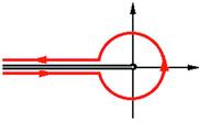
Figure 14.12 Contour for representation (14.81) of Bessel function ![]() of noninteger order.
of noninteger order.