Chapter 3
Getting Creative with the Canvas
The canvas is one of the most exciting new elements in HTML5—perhaps the most exciting. Not only does it provide a powerhouse of visual specialties, but it is also competition for Adobe Flash. I say that with a grain of salt (and a slice of lemon). Flash is a monster of a tool/utility/product—call it what you will. Flash has brought the web site experience to new heights for those sites that make use of it.
However, the use of Flash has been sidetracked with a whammy of a dilemma. At the time of this writing, Flash does not work in Apple mobile devices: the iPad and iPhone. Is this a good or bad thing for Apple? For Adobe (which makes Flash), it is clearly a negative. As developers, we can stay out of the way of that business entanglement and deal with it on our level by using HTML5 in place of Flash. With the canvas in HTML5, we can skirt the issue. The canvas is native HTML. It is not a plug-in, add-on, or something that you must download.
At some point, all browsers will fully support the canvas (yes, a rub on Internet Explorer here). The canvas is core to HTML5 and raring to go. So let’s get to it.
Introducing the Canvas
As with any introduction to a technology, the old standard “Hello World” is typical to see. Here, I’ll show you the equivalent. You will not see the words “Hello World.” You will not see any words at all. What you will see is a canvas sitting on a web page. It has a border and a background color, but is essentially blank and unexciting, yet it is there, or rather here—in Figure 3-1.
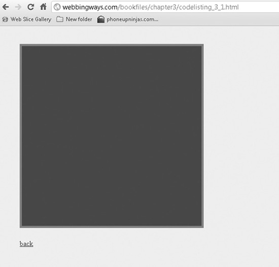
Figure 3-1 Say hello to the canvas
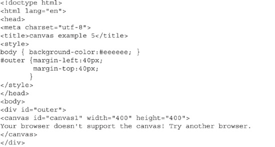
This plain canvas does nothing other than be visible. In this chapter and the next, we will add drawing, animation, and event usage. To get started, we’ll simply display the canvas, as in Figure 3-1. Code Listing 3-1 shows the source code that presents the canvas on the web page.
Code Listing 3-1 Displaying a canvas element
A simple code construct is all it takes to display a canvas:

As with other HTML elements, you use an opening tag and a closing one. In the case of the canvas, a line of text informing the user that the browser does not support showing the canvas is placed between the opening and closing tags. This informative line appears when the canvas itself cannot be displayed (as we wait for all browsers catch up with technology). Otherwise, the canvas will appear.
A line of text stating that a browser does not support the canvas will appear when that case is true; otherwise the canvas will appear. The text statement goes in between the opening and closing tags of the canvas.
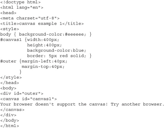
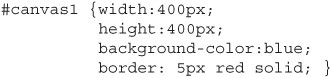
The canvas is styled a bit with a red border and a blue interior, as well as given a width and height:
Drawing on the Canvas
Common among drawing programs is the ability to place shapes, free-form lines, and usually something along the lines of layering. The canvas makes use of the Red, Green, Blue (RGB) model of color representation, which has been around for a long time. It also has a variation that includes the alpha channel, for setting transparency. The acronym now becomes RGBA. It is not required to include the fourth (alpha) component to indicate color; in other words, RGB and/or RGBA can be used.
Code Listing 3-2 displays a few rectangles on the canvas. One rectangle does not use transparency, and the rest do use it.
Code Listing 3-2 A canvas showing rectangles
So, what does it look like? See Figure 3-2. First, the canvas element is coded as follows:
![]()
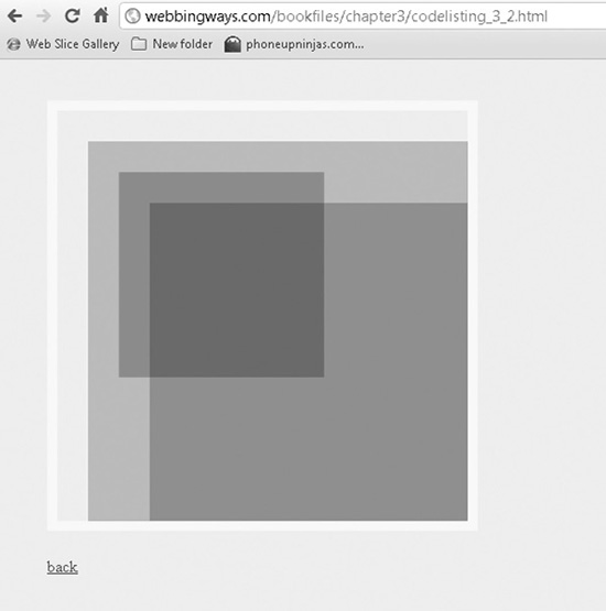
Figure 3-2 A canvas displaying rectangles
In this case, the width and height are put directly in-line with the element tag.
Displaying the canvas is pretty much just a line of code, as you’ve seen. The action is in the use of JavaScript. An application programming interface (API) is built into the canvas. It needs to be declared, and is known as the context. Indeed, the code that brings it to the plate is getContext:
![]()
Currently, there is one type of context, which sets up a two-dimensional drawing surface. An approach to simulate 3D is shown in the book’s last chapter.
Once the canvas and the context are established, which is done here with variables (mycanvas and cntx), other activities, such as drawing, can occur. The context provides the hook to the API, which has methods for image manipulation on a two-dimensional plane.
Two approaches are available for putting shapes on a canvas:
![]() Stroke is used for creating the edges of a shape.
Stroke is used for creating the edges of a shape.
![]() Fill is used to fill the interior.
Fill is used to fill the interior.
In the example in Figure 3-2, the rectangles are filled. So, using the established context variable (cntx in this case), the fillStyle and fillRect methods are used. The first sets the color using RGB, and the second sets the position and size of the rectangle. The background color of the canvas is gray, as indicated for the overall page color (given to the body tag) A solid purple rectangle is placed on top of this, beginning at a top and left position of 30 pixels offset from the canvas border, and extending to the bottom-right corner, indicated by the 400, 400 setting. The size of the canvas is 400 × 400, so this rectangle is taken to that lower-right corner:
![]()
Note that when either rgb or rgba is used, the setting is enclosed in either single quotes or double quotes.
Next, a rectangle is drawn with full green and blue, which results in a green-blue color. However, here the alpha channel is used to set the transparency at 50%. Therefore, the color of the rectangle is altered by both the purple one under it and the black one over it. The black rectangle does not look black at all, but more on that in a moment. Here is the code for the 50% transparent rectangle:
TIP
Transparency is set by placing a value between 0 and 1 in the RGBA construct. The use could seem backward. The setting is not actually an indication of the transparency percent, but rather of the solidity percent. For example, 0.2 indicates just 20% is visible, not that 20% is transparent.
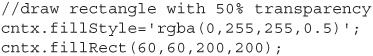
This rectangle is smaller based on the dimensions given. The next rectangle is larger. It is set to black—an RGB of 0,0,0 ('rgba(0,0,0,0.25)'); however, the transparency is set to just 25%, which can be confusing. This really means it’s 75% transparent. As such, its black color does not have the rectangle clearly cover the large portion of the canvas. At best, it just makes the other rectangles a bit darker in the converged area. To make this clear, the canvas shown in Figure 3-3 is altered to have the rectangle appear with just 25% transparency (the amount in the RGBA is set to .75). The rectangle is now much darker and covers up much more of the underlying rectangles.
Figure 3-3 The rectangle’s transparency setting is changed.
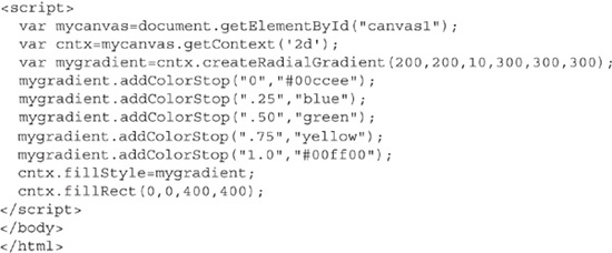
Using Gradients
Gradients are visuals that mix two or more colors. The colors don’t mix in the sense that red and blue make purple. Instead, the colors are set at points, and the variation of the mix smoothly transitions from one color to the other, similar to how a rainbow appears. For example, picturing a square, red could be on one side and blue on the other. Along the width of the square (or the height, depending on the orientation), the coloring is seen as smoothly changing from red to blue. Figure 3-4 illustrates this with a square that is all red on the left and all blue on the right.
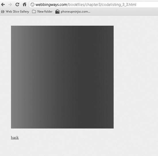
Figure 3-4 A simple gradient
Gradients are established by using a method that creates the gradient along with color stops. The gradient has four settings: the left, top, bottom, and right points (relative to the canvas). A color stop has two parts: a positional offset relative to the coordinates established by the gradient method and the color setting itself. Two gradient types are available: linear and radial.
Code Listing 3-3 shows the code that creates the image in Figure 3-4.
Code Listing 3-3 A simple gradient
Here are the lines of code that create the gradient:
The context to the API is set (cntx). Then a variable (mygradient) is set to one of the gradient types. Here, it is the linear gradient. Using the variable, the color stops are added. The addColorStop method is applied to the gradient variable, once for each color stop. The color stop takes two parameters. First is a positioning in the gradient, using a value between 0 and 1. The second parameter sets the color. You can use any number of color stops, although practical use should keep the number to something subjectively reasonable. A gradient with an excessive amount of color stops will likely appear as a squeezed bunch of colors without smooth transitions.
Finally, the fill style (fillStyle) method of the context is applied to the variable holding the gradient settings, and a fill method (fillRect) is used to complete the rectangle. If it helps, think of this as “create gradient, set colors, and fill it.”
Linear Gradients
Linear gradients follow a straight path from one color to another. A linear gradient can have several colors, each set with a different position along the way. This provides numerous possibilities for how a linear gradient will appear. Figure 3-5 shows a linear gradient with five color stops. Code Listing 3-4 shows the code used to create this figure.
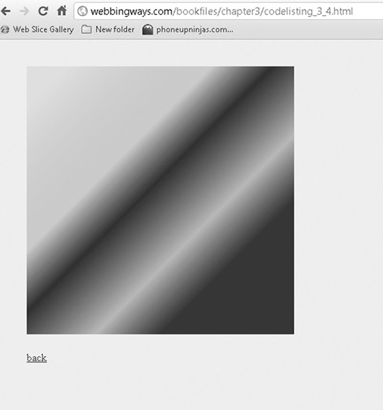
Figure 3-5 A linear gradient with five color stops
Code Listing 3-4 A complex linear gradient

Each of the five color stops is sequentially in position from 0 to 1, along with its associated color. The gradient itself is created with the createLinearGradient method:

Even with the the color stops set to span from 0 to 1, the gradient is also set to sit at coordinates 30, 30 to 300, 300 on top of a canvas that is 400 × 400 pixels. The four linear gradient coordinates are set in the createLinearGradient method. The first color stop establishes a yellow color (#ffdd30), and the last color stop establishes a gray color (#333333). Logically then, the canvas is filled with these colors from its corners to where these color stops sit.
TIP
If the coordinate system in unfamiliar, think of graph paper. In some systems, the center point would relate to position 0, 0. Here the 0, 0 position is the upper-left corner.
Radial Gradients
Radial gradients appear to spread from a point outward. The method to make one, createRadialGradient, takes six parameters, unlike the createLinearGradient method, which takes only four parameters. The six parameters of the radial gradient are best thought of as two sets of three parameters, with each set establishing the starting point and the radius of a circle. By setting the circles with different parameters, the radial effect is created, as shown in Figure 3-6.
Notice how the radial gradient can appear to not fit completely on the canvas. This effect is caused by the parameter used to create the gradient. Code Listing 3-5 shows the code used to create the radial gradient shown in Figure 3-6.
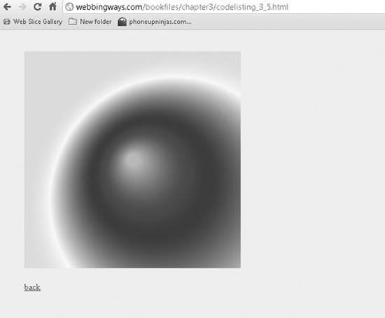
Figure 3-6 A radial gradient
Code Listing 3-5 A radial gradient
As with linear gradients, color stops are used as points to vary the color. The parameters used to create this gradient set up two circles. One is centered at the coordinates 200, 200 with a radius of 10, and the other is centered at the coordinates 300, 300 with a radius of 300. Since the second circle starts in the lower-right quadrant of the canvas (which itself is 400 × 400), and the circle has the radius of 300, it is larger, at least based on its starting place, to fit on the canvas.
NOTE
A radius is a straight line extending from the center of a circle to the edge of the circle.
Understanding Paths
You can draw on a canvas by using one or more drawing methods. The examples shown so far in this chapter required the appropriate method, such as fillRect or createRadialGradient. These methods are straightforward in that they create the item along with taking a parameter for size or placement.
Other drawing methods make use of paths. Paths have a beginning and end based on code statements (beginPath and closePath). These are best described as organizational points that provide a way to make distinctive blocks of drawing statements. In some cases, they are necessary, as a drawing method may continue to draw from where the last drawing method left off. This becomes obvious in drawing lines, especially when several lines are combined to make a custom shape or other visual. Here’s a quick example of a code construct to draw a circle:
Drawing Circles and Arcs
Circles and arcs are both created with the same method: arc. The parameters make the difference for how the shape appears. Here’s an example that creates a circle:
![]()
The following creates an arc (in this case, a semicircle):
![]()
The parameters, in order, are the left position, the top position, the radius, the start angle, the end angle, and the direction. Left and top together indicate a point, or coordinate position. The radius controls how large the arc will be. Concerning the two angle settings, consider that a circle has 360 degrees. If you were to put a pen on paper and draw a quarter-circle, you would be completing an arc covering 90 degrees. However, did you draw this quarter-circle from a true 0-degree position (for example, the 12:00 position on a clock) to a true 90-degree position (for example, the 3:00 position on a clock)? Or did you draw it from, say, the 250-degree position to the 340-degree position? Either approach would account for a coverage of 90 degrees. The angle settings determine where the drawing of the arc starts and stops using this methodology.
However, the start angle and end angle settings work with radians, not degrees. Radians are an alternate measurement system. How many radians make a complete circle? The answer is 2 times pi, or approximately 6.28. Therefore, the start and end angles should be from 0 to 6.28.
A start of 0 and an end of pi times 2 creates a complete circle. A shorter range (for example, 0 and 4) creates a portion of a circle. A start angle value of 0 actually indicates starting at the 3:00 position (not the probably assumed 12:00 position). It is perfectly fine to indicate starting at 1 or another number.
The last parameter indicates whether the arc is drawn clockwise or counterclockwise. False (the default if left out) draws in a clockwise direction. True draws in a counterclockwise direction. Experimenting with different values for the start and end angles, and toggling true and false of the last parameter will show how it comes together.
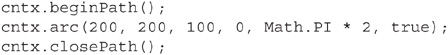
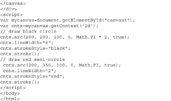
Code Listing 3-6 shows the circle (angles range of 0 to pi times 2), semicircle (angles range of 0 to pi), and the use of beginPath and closePath.
Code Listing 3-6 A circle and an arc
To draw a circle, multiply pi × 2, as in the following:
![]()
Code Listing 3-6 draws a circle. It is a complete circle, since pi is doubled in the appropriate parameter:
![]()
Conversely, a semicircle is created when pi is the value used:
![]()
Of course, seeing it makes it clear. Figure 3-7 shows the circle and semicircle created with Code Listing 3-6.
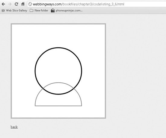
Figure 3-7 Drawing circles and arcs
Figure 3-8 illustrates what happens when the beginPath and endPath statements are removed. As you can see, the use of the path statements affect how an image is drawn. Code Listing 3-7 is the source for the image in Figure 3-8.
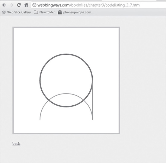
Figure 3-8 Altering the image by removing the path statements
Code Listing 3-7 An altered arc
Trying different values for the parameters in the arc method provides different shapes. They will still have the circle/part-circle appearance, but with some experimentation, you can achieve some interesting variations, as shown in Figure 3-9.
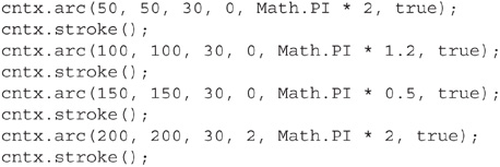
Code Listing 3-8 shows the source for the image in Figure 3-9. Note the varied parameters in each cntx.arc() statement.
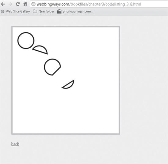
Figure 3-9 Arc variations
Code Listing 3-8 Varied circular shapes


Working with arcs, you can also show the image as one continuous line by removing the path statements. The middle section of code in Code Listing 3-8 becomes this:
NOTE
The output is identical if you do not have any beginPath … closePath statements or if you enclose the entire middle section in one beginPath … closePath statement.
Figure 3-10 shows the change in the image after removing the path statements.
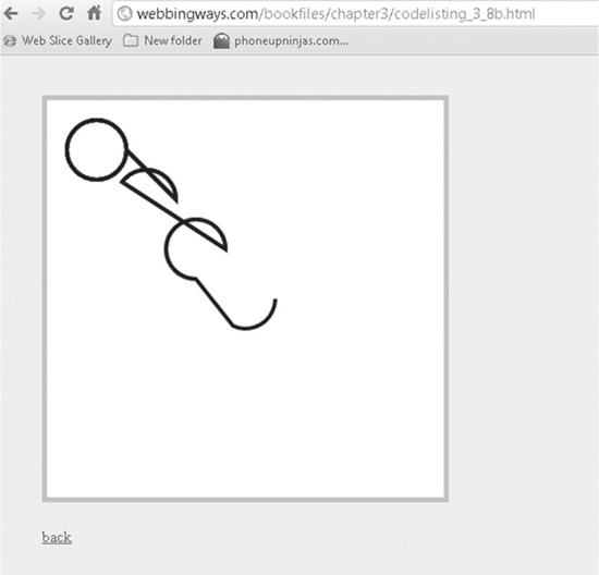
Figure 3-10 Continuous line arcs
Figure 3-11 shows a canvas filled with small circles. If each were individually coded within a path block, it would be a rather long listing of code. The point here is not the drawing technique (they are just circles), but rather it’s the JavaScript used to do this. JavaScript looping is put to work to make the circles. The full code for this example is shown in Code Listing 3-9.
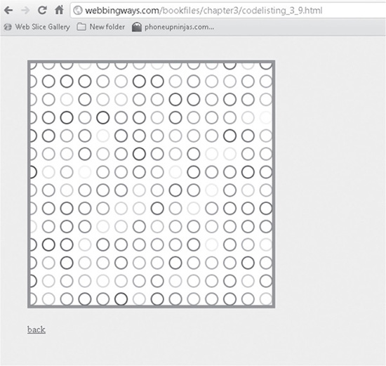
Figure 3-11 Many circles on a canvas
Code Listing 3-9 Using JavaScript looping to make circles
The pertinent part of the code used to make the circles is this:
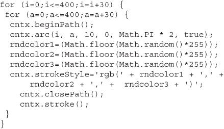
What you see here is a set of loops, one nested in the other. One loop sets the left parameter, and one sets the top parameter. The order in which these loops occur in this example is not important, since they are both the same size; in other words, they each iterate the same number of times. Also, they increment by the same amount (30). Within the nest of loops, a beginPath method is stated, and then the arc method is used with PI * 2 (to make the arc a circle). Next, three random colors are established to use in the RGB color construct, which happens next in the strokeStyle method. This method is used to set the color. Then the path is closed. Finally, the circle is drawn with the stroke method.
This occurs repeatedly until the loops run out. On the canvas, 196 circles are placed—or about 196, since the increment of 30 does not fit exactly with the 400 × 400 dimension of the canvas. This results in some circles being cut off.
Since the colors are selected using JavaScript’s random method, each refresh of the browser shows a different spread of color among the circles. Later in the chapter, you will see these circles again in a way that uses an animation technique to continuously change the colors.
Drawing Lines
Rectangles, circles, arcs, and other predefined shapes are great, yet when it comes to drawing, the ability to create a line is paramount. The two main methods for drawing lines are moveTo and lineTo. Imagine a pen pressed down on a piece of paper. If you move the pen, a line is drawn; if you keep the pen down but draw in a different direction, another line is drawn, and it is connected to the first line. What if you need to start a new line somewhere else that is not connected? Then you need to lift the pen and move it. The lineTo and moveTo methods are how you achieve these actions.
Figure 3-12 shows a house drawn with a number of lines, connected and not connected, as well as a round doorknob to boot (made with the arc method).
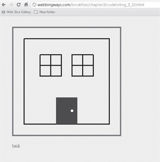
Figure 3-12 A house drawn with the moveTo and lineTo methods
The code used to make this image uses reusable JavaScript functions and a number of techniques. An overview of the code is shown in Code Listing 3-10.
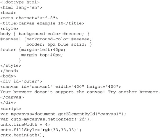
Code Listing 3-10 Drawing lines
Keep in mind that a line has a starting position and an ending position. The coordinate system is in play here. The starting position has two numbers (left and top), while the ending has another two (also left and top).
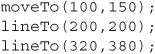
The starting position can be determined either by the moveTo method or by being implied by where the drawing last took a pause, which must be at some set of coordinates. The only difference is whether you first lifted the pen. If so, you used the moveTo method. Therefore, moveTo(100,150) places the pen down at a position of 100 pixels in from the left and 150 pixels down from the top. If this were followed by a lineTo(200,200), a line would be drawn from the designated position to the 200, 200 spot. If this were then followed by lineTo(320,380), a line would be drawn from 200, 200 to 320, 380. That second draw action assumed the last stopped spot of 200, 200 as the place to start from. Had there been another moveTo (which is like lifting the pen), it would designate the starting point. But as described here, there was no second moveTo. So, here is what we have from this example:
Besides this, no lines are drawn unless there is a stroke method used.
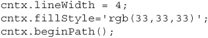
Let’s dissect the code in Code Listing 3-10 (no, not quite like a biology class). First, a line width and color are selected. The 'rgb(33,33,33)' sets a fairly dark color, approaching black. Then a beginPath statement is put in.
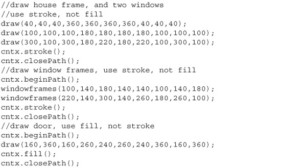
After the path is opened, drawing is performed. In this example, a function named draw() is used. This function accepts a slew of variables to do the work. It takes ten parameters. The first two are used for the moveTo method, and the other eight are actually four sets of two parameters used with four successive lineTo methods. Thinking this through, imagine a pen is put down on a piece of paper, and a square is drawn. A square has four sides—the four successive lineTo iterations.
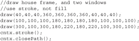
Notice that after the beginPath started a path block, the draw method is called three times in a row. Then a single stroke method call draws all three squares, and a final closePath is stated. The draw method is shown in the following code.
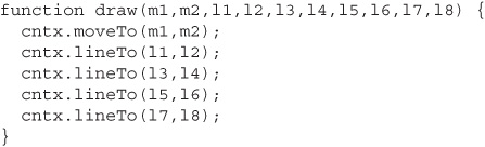
First, for clarity, the eight parameters are each the letter l (for line), followed by a number. The first two parameters place the pen using moveTo, and then following are the four iterations of lineTo. If you closely follow the parameters sent to the function, like this:
![]()
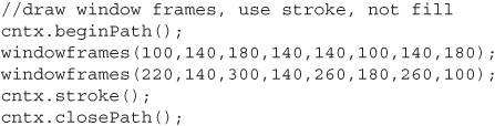
you’ll see a square is drawn. The three successive calls to the draw method draw the large frame around the house (not to be confused with the border of the canvas), and also draw the two windows—just squares for the moment, without cross frame lines in them.
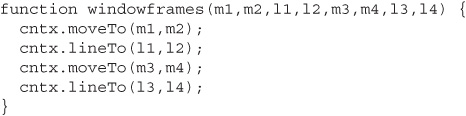
Next, the crosses on the windows are drawn in much the same way as the squares; that is, parameters are sent to a function, named windowframes() in this case.
The windowsframe function has fewer parameters. The first pair are moveTo coordinates, the second pair are for a lineTo, the third pair is for another moveTo, and the last pair is for another lineTo. Here is the actual function:
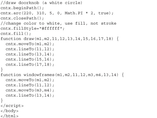
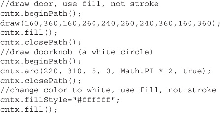
Rounding out the picture are the door and doorknob. The door is drawn with the draw function. However, upon returning from the function, a fill is used instead of a stroke. This means the drawn rectangle of the door is filled in, not outlined like the windows. Finally, an arc method places the doorknob—a small, white circle—and it becomes visible with a fill. Just prior to the fill, the color is changed to white with the fillStyle method.
This one comprehensive example of drawing a house should suffice for demonstrating how drawing works. You’ve seen how it relates to what you do when drawing on a piece of paper.
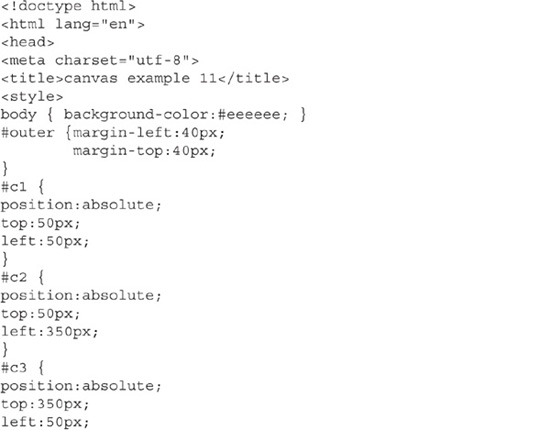
Using Multiple Canvases
This is fun—a page filled with multiple canvases, each doing its own thing. Since each canvas can be named individually, each can be treated separately with CSS and JavaScript. Figure 3-13 shows four canvases on a single web page.
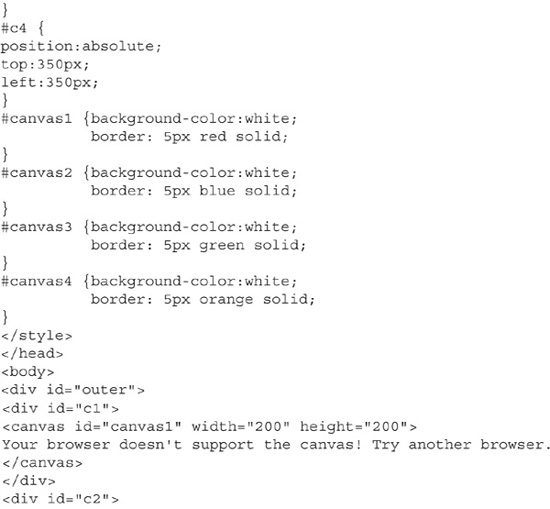
Code Listing 3-11 shows how each canvas is inside its own div, as well as being uniquely named. CSS is applied to both the divs and the canvases. CSS is used for page placement and canvas border colors.
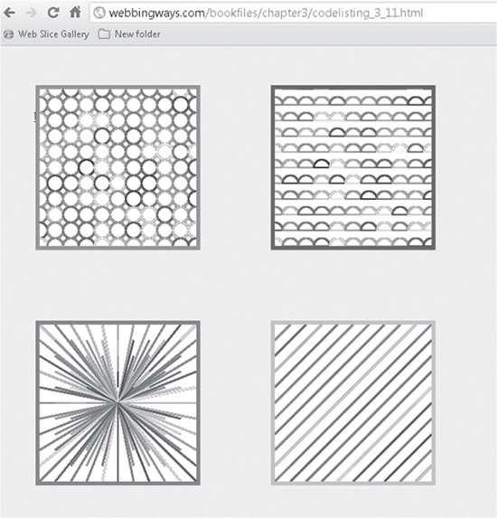
Figure 3-13 Multiple canvases on a single web page
Code Listing 3-11 Multiple canvases
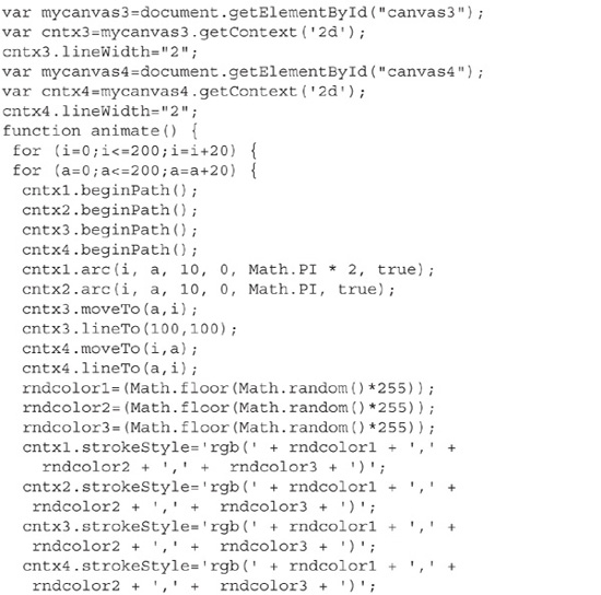
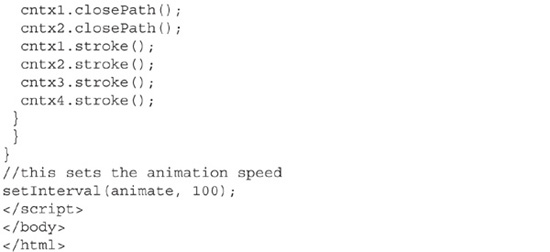
This code uses many techniques already discussed in this chapter. Of note is the large function (animate) in the middle. What is different here is how the function is called. The JavaScript setInterval method is used to repeatedly call the function:
![]()
A setting of 100 indicates to call the function every tenth of a second. At a fairly fast speed, the canvases are all showing an animated view. To see this in action, visit www.webbingways.com or www.mhprofessional.com/computingdownload.
Placing Text on a Canvas
So far, you’ve seen examples of visual images placed on a canvas. What about text? Can words be placed on a canvas? Of course! There are many methods to work with text, including textAlign, measureText, textBaseline, font, fillText, and strokeText. The fillText and strokeText methods are used to affect whether alphanumeric characters are outlined or filled in.
The example in Code Listing 3-12 shows a technique in which the canvas is filled with a line of text repeatedly.
Code Listing 3-12 Lines of text
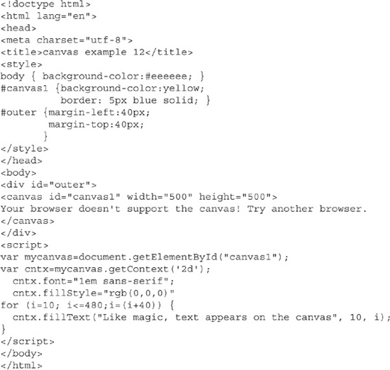
The code in Code Listing 3-12 uses the font setting of the context to declare a sans-serif font sized at the standard 1em. The fillStyle method sets the color to black. The fillText method puts the text on the canvas.
The fillText method takes three parameters: the text, the left position, and the top position. In this example, the top is looped downward to create the effect of filling the canvas with the text, as shown in Figure 3-14.
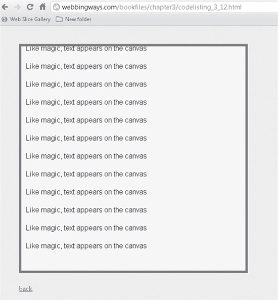
Figure 3-14 Sequential text
Vertical Text
Text is placed on the canvas using a method that specifies a coordinate for where the text is to begin. With a little ingenuity, this can be made to accommodate vertical text by placing each letter underneath the one that came before it. Figure 3-15 shows how this looks.
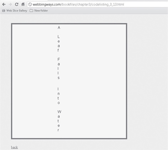
Figure 3-15 Vertically oriented text
Code Listing 3-13 shows the vertical text technique. In the code, a function named letter() is used to place the text. Single characters and their vertical position are passed to the function.
Code Listing 3-13 Vertical text
The letter function in Code Listing 3-13 is passed only two parameters: the alphanumeric character and the vertical position to place it. The horizontal position is fixed at 200 pixels. This forces all letters to be underneath each other in a vertical line.
Shadow Text
Text can be stroked or filled—in other words, be an outline of letters or filled in. This offers possibilities of creating shadow effects with either type of text. It all has to do with placement and transparency. First, text that is outlined by using strokeText is placed on the canvas and duplicated with a slight offset to create a shadow. The direction, length, and transparency of the shadow can be controlled with the available features of the various canvas methods. Figure 3-16 shows an example using stroked text. Code Listing 3-14 shows the code used to produce this effect.
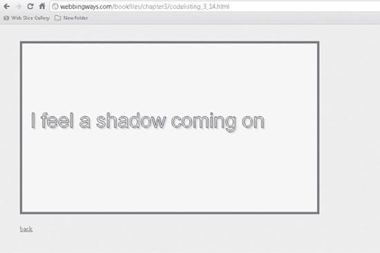
Figure 3-16 Creating a text shadow
Code Listing 3-14 Outlined, shadowed text
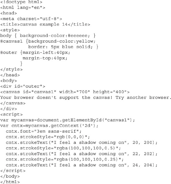
This example uses a large text size since it is stroked and not filled. The basic line of text is placed at the coordinates of 20 pixels to the left, and 200 pixels down, relative to the canvas. This line of text has a solid outline. Following this are two more lines of text. The text is identical, however the offsets are sequentially 2 pixels to the bottom and right. With each of the lines, the transparency increases as well, creating the shadow effect.
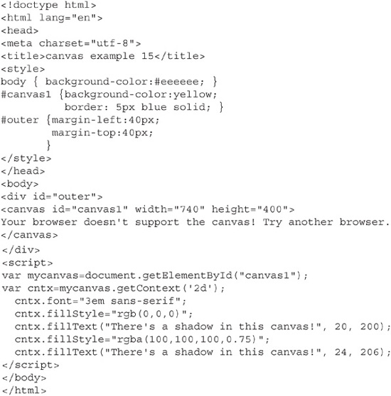
Filled text can also be shadowed quite effectively. The same approach applies. Display a line of text, and then display and offset with a given transparency. Figure 3-17 shows how this looks with filled text.
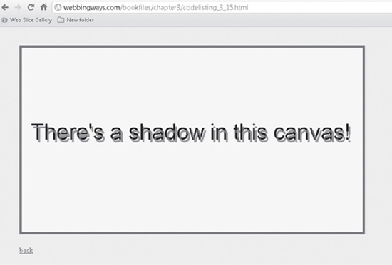
Figure 3-17 Filled, shadowed text
The image in Figure 3-17 displays the shadow with a 4-pixel offset to the bottom and the right. The transparency is slight—just 25% is on the alpha channel. Code Listing 3-15 shows how the image is made.
Code Listing 3-15 Filled, shadowed text
You can apply creative techniques with shadows. For example, the shadow can be a different color, or the shadow can use several offsets with increasing transparency until the text completely disappears. Experiment! This is one great way to put pizzazz in your pages.
Summary
The canvas is an exciting and versatile addition to HTML. As a container, in essence, it can display many types of visuals. This chapter has introduced how to work with basic shapes, gradients, ways to draw, and text. But that’s not all!
The examples in this chapter have been static for the most part (some animation was demonstrated). In Chapter 4, you’ll learn how to use animation and events. If you feel comfortable with what you’ve seen so far, please dive right in!