Let's take a step back and define some terminology. A graph is a structure comprising of nodes (also called vertices) that are connected by links called edges . Depending on the type of graph, the edges may be bidirectional or unidirectional and may have weights associated with them. For example, a city road network can be seen as a graph where the roads are the edges, and intersections and points of interest are nodes. Some streets are one-way and some are not, some have tolls, some are closed at certain times of day, and so forth.

For transportation companies, there is much money to be made by optimizing the routes taken from one point to another. Different graph algorithms can derive such routes by taking into account attributes such as one-way streets and other costs expressed as weights that make a given road more attractive or less so.

For a more current example, think of the social graph popularized by sites such as Facebook where the nodes are people and the edges are the relationships between them.

The main reason graphs don't look like many other MapReduce problems is due to the stateful nature of graph processing, which can be seen in the path-based relationship between elements and often between the large number of nodes processed together for a single algorithm. Graph algorithms tend to use notions of the global state to make determinations about which elements to process next and modify such global knowledge at each step.

In particular, most of the well-known algorithms often execute in an incremental or reentrant fashion, building up structures representing processed and pending nodes, and working through the latter while reducing the former.

MapReduce problems, on the other hand, are conceptually stateless and typically based upon a divide-and-conquer approach where each Hadoop worker host processes a small subset of the data, writing out a portion of the final result where the total job output is viewed as the simple collection of these smaller outputs. Therefore, when implementing graph algorithms in Hadoop, we need to express algorithms that are fundamentally stateful and conceptually single-threaded in a stateless parallel and distributed framework. That's the challenge!

Most of the well-known graph algorithms are based upon search or traversal of the graph, often to find routes—frequently ranked by some notion of cost—between nodes. The most fundamental graph traversal algorithms are depth-first search (DFS) and breadth-first search (BFS).The difference between the algorithms is the ordering in which a node is processed in relationship to its neighbors.

We will look at representing an algorithm that implements a specialized form of such a traversal; for a given starting node in the graph, determine the distance between it and every other node in the graph.

The first problem we face is how to represent the graph in a way we can efficiently process using MapReduce. There are several well-known graph representations known as pointer-based, adjacency matrix, and adjacency list. In most implementations, these representations often assume a single process space with a global view of the whole graph; we need to modify the representation to allow individual nodes to be processed in discrete map and reduce tasks.

We'll use the graph shown here in the following examples. The graph does have some extra information that will be explained later.

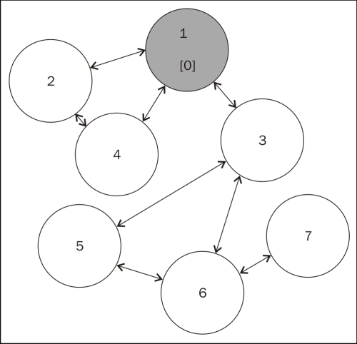
Our graph is quite simple; it has only seven nodes, and all but one of the edges is bidirectional. We are also using a common coloring technique that is used in standard graph algorithms, as follows:

As we process our graph in the following steps, we will expect to see the nodes move through these stages.