Chapter Nine

Moment-Generating Function

9.1 Introduction/Purpose of the Chapter

We chose to introduce the generating function and the moment-generating function after the chapter on characteristic function. This is contrary to the traditional and historical approach. In modern-day probability the characteristic functions are much more widespread simply because they exist and can be constructed for any random variable or vector regardless of its distribution. On the other hand, generating functions are defined only for positive discrete random variables. The moment-generating function does not exist for many discrete or continuous random variables. Despite this fact, when these functions exist, they are much easier to work with than the characteristic functions (recall that the characteristic function takes values in the complex plain). Thus, we feel that the knowledge of these functions cannot miss from the culture of anyone applying probability concepts.

9.2 Vignette/Historical Notes

According to Roy (2011), Euler found a generating function for the Bernoulli numbers around 1730's. That is, he defined numbers B_n such that

Around the same time, DeMoivre independently introduced the method of generating functions in a general way (similar to our definition). He used this method to encode all binomial probabilities in a simple polynomial function. Laplace (1812) applied the Laplace transform to probability, in effect creating the moment-generating function. 281

9.3 Theory and Applications

9.3.1 Generating Functions and Applications

First, we introduce a generating function for discrete probability distributions. This function in fact can be defined for any sequence of numbers.

Definition 9.1. (Regular generating function) Let a = {a_i}_i{0,1,2,...} be a sequence of real numbers. Define the generating function of the sequence a as

The domain of definition of the function G_a(s) is made of values for which the series converges.

---

Remark 9.2 Please note that we can obtain all the terms of the sequence if we know the generating function. Specifically,

where we denote with the i-th derivative of the function G_a calculated at x₀.

---

Example 9.1 A simple generating function

Take the sequence a as

Then its generating function is

provided that the power term converges to 0. This holds if |s| < 1 for all α; and obviously the radius of convergence may be increased, depending on the value of α. The DeMoivre theorem may be proven easily by taking derivatives of this expression and calculating them at s = 0.

---

Definition 9.3 The convolution of two sequences {a_i} and {b_i} is the sequence {c_i} with

We write c = a ∗ b.

---

Lemma 9.4 If two sequences a and b have generating functions G_a and G_b, then the generating function of the convolution c = a ∗ b is

---

Proof: We have

9.3.1.1 Generating Functions for Discrete Random Variables

Definition 9.5 (Probability generating function(discrete)) If X is a discrete random variable with outcomes and corresponding probabilities p_i, then we define

This is the probability-generating function of the discrete random variable X.

---

Lemma 9.7 Suppose that two independent discrete random variables X and Y have associated probability distributions p = {p_n} and q = {q_n} and generating functions G_X(s) = ∑ _isⁱp_i and G_Y(s) = ∑ _isⁱq_i respectively. Then the random variable X + Y has distribution the convolution of the two probability sequences p ∗ q as in Definition 9.3.3 and its generating function is

---

Proof. The proof is an exercise. Just use the preceding lemma and calculate

in terms of p_i and q_i.

This definition and the lemma above explain the main use of the generating functions. Recall that the probability distribution may be recovered entirely from the generating function. On the other hand, the generating function of a sum of two random variables is the product of individual generating functions. Thus, while the distribution of the sum using the convolution definition is complicated to calculate, calculating the generating function of the sum is a much simple process. Once calculated, the probability distribution of the sum may be obtained by taking derivatives of the generating function.

Proposition 9.8 (Properties of probability-generating function) Let G_X(s), G_Y(s) be the generating functions of two discrete random variables X and Y.

i. There exists R ≥ 0, a radius of convergence such that the sum is convergent if |s| < R and diverges if |s| > R. Therefore, the corresponding generating function G_X exists on the interval [− R, R].

ii. The generating function G_X(s) is differentiable at any s within the domain |s| < R.

iii. If two generating functions G_X(s) = G_Y(s) = G(s) for all |s| < R where R = min {R_X, R_Y}, then X and Y have the same distribution. Furthermore, the common distribution may be calculated from the generating function using

iv. As particular cases of the definition, we readily obtain that

The last relationship implies that the probability-generating function always exists for s = 1, thus the radius of convergence R ≥ 1.

---

Proof: Exercise 9.8.

9.3.1.2 Generating Functions for Simple Distributions

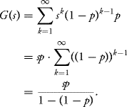
Bellow we present the generating function for commonly encountered discrete random variables.

Once again we stress that the generating functions are very useful when working with discrete random variables (basically when they exist).

Lemma 9.9 If X has generating function G(s), then:

i. E(X) = G′(1).

ii. E[X(X − 1) (X − k + 1)] = G^(k)(1), the k-th factorial moment of X.

---

Proof. Again these results are easy to prove and are left as exercises.

9.3.1.3 Examples

In the next examples we show the utility of the generating functions.

Solution: We could compute the convolution f_Z = f_X ∗ f_Y using the formulas in the previous section. However, calculating the distribution using generating functions is easier. We have

By independence of X and Y and from the Lemma 9.3.7 above, we have

But this is the generating function of a Poisson random variable. Identifying the parameters imply that Z has a Poisson(λ + μ) distribution.

Example 9.3 Using Generating Function for Binomial Distribution

We know that for a Binomial(n, p) random variable X may be written as X = X₁ + + X_n, where X_i's are independent Bernoulli(p) random variables. What is its generating function? What is the distribution of a sum of binomial random variables?

---

Solution: Again applying the Lemma 9.7, we obtain the generating function of a Binomial(n, p) as

What if we have two independent binomially distributed random variables X Binomial(m, p) and Y Binomial(k, p)? Note that p the probability of success is identical. What is the distribution of X + Y in this case?

We see that we obtain the generating function of a Binomial random variable with parameters m + k and p.

This is of course expected. If X can be written and a sum of n Bernoulli(p) and Y can be written along with a sum of k Bernoulli(p), then of course X + Y is a sum of n + k Bernoulli(p) random variables. Even more intuitively, suppose X is the number of heads obtained in n tosses of a coin with probability p, and Y is the number of Heads obtained in k tosses of the same coin (separate tosses). Then of course X + Y is the total number of heads in n + k tosses.

Let us expand this results in which we presented the distribution of a sum of a fixed number of terms. Consider the case when the sum contains a random number of terms. The next theorem helps with such a situation.

Theorem 9.10 Let X₁, X₂, ... denote a sequence of i.i.d. random variables with generating function G_X(s). Let N be an integer-valued random variable independent of the X_i's with generating function G_N(s). Then the random variable

has generating function:

---

Now let us give an example of application of the previous theorem.

Solution: We know that

The last distribution is the distribution of the number of eggs hatching if we know how many eggs were laid.

We may then calculate the conditional expectations. Let

since that is the formula for the expectation of a Binomial(n, p) random variable. Therefore, E(K|N) = ϕ(N) = Np. Recall that E[E[X|Y]] = E[X]. Using this relation, we get

To find E(N|K), we need to find f_N|K:

if n ≥ k and 0 otherwise, where q = 1 − p and for the denominator we have used the following:

since P(K = k|N = m) = 0 for any k > m (it is not possible to hatch more chicks than eggs laid).

Consequently, we immediately obtain

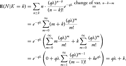
which gives us E(N|K) = qλ + K.

Note that in the previous derivation we kind of obtained the distribution of K. We still have to calculate a sum to find the closed expression. Even though this is not that difficult, we will use generating functions to demonstrate how easy it is to calculate the distribution using them.

Let K = X₁ + + X_N, where the X_i ~Bernoulli(p). Then using the the above theorem, we obtain

Using the above equations, we conclude that

But since this is a generating function for a Poisson r.v., we immediately conclude that

Solution: Exercise. Please read and understand the previous example.

9.3.2 Moment-Generating Functions. Relation with the Characteristic Functions

Generating functions are very useful when dealing with discrete random variables. To be able to study any random variables, the idea is to make the transformation s = e^t in G(s) = E(s^x). Thus, the following definition is introduced.

Definition 9.11. (Moment-generating function The moment-generating function of a random variable X is the function given by

defined for values of t for which M_X(t)< ∞.

---

The moment-generating function is related to the Laplace transform of the distribution of the random variable X.

Definition 9.12 (Laplace transform of the function f) Suppose we are given a positive function f(x). Assume that

for some value of x₀ > 0. Then the Laplace transform of f is defined as

for all t > t₀. If the random variable X has distribution function F, the following defines the Laplace–Stieltjes transform:

again with the same caution about the condition on the existence.

---

With the previous definitions it is easy to see that the moment-generating functions is a sum of two Laplace transforms (provided either side exists). Specifically, suppose the random variable X has density f(x). Then,

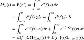
where

and

This result is generally needed to use the theorems related to Laplace and specially inverse Laplace transforms.

Proposition 9.13 (Properties) Suppose that the moment-generating function of a random variable X, M_X(t) is finite for all .

i. If the moment-generating function is derivable, then the first moment is ; in general, if the moment generating function is k times derivable, then .

ii. More general, if the variable X is in L^p (the first p moments exist), then we may write (Taylor expansion of e^x):

iii. If X, Y are two independent random variables, then M_X+Y(t) = M_X(t)M_Y(t).

---

Example 9.6 Calculating Moments Using the M.G.F.

Let X be an r.v. with moment-generating function

Derive the expectation and the variance of X.

---

Solution: Since

we get for t = 0 and Proposition 9.13

By differentiating M_X, twice, we obtain

and

Thus

Let us compute the moment-generating function for certain common probability distribution.

Proposition 9.16 Suppose X ~ N(0, 1). Then

for every .

---

Proof: For every , we have

Proposition 9.17 If X ~ N(μ, σ²), prove that for every , we have

---

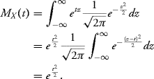
Proof: See problem 9.3.

Proposition 9.18 If X ~ Exp(λ) with λ > 0, then

---

Proof: See exercise 9.5.

Proposition 9.19 If X ~ Γ(a, λ) (gamma distribution with parameters a, λ > 0), then the moment-generating function M_X exists for t < λ and in this case we have

---

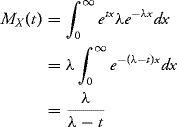
Proof: By the definition of the gamma density, we have

Use the change of variables y = x(λ − t) to conclude.

9.3.3 Relationship with the Characteristic Function

If the moment-generating function of a random variable X exists, then we obviously have

We recall that just as the moment-generating function is related to the Laplace transform, the characteristic function was related to the Fourier transform.

We note that the characteristic function is a better-behaved function than the moment-generating function. The drawback is that it takes complex values and we need to have a modicum of understanding of complex analysis to be able to work with it.

9.3.4 Properties of the MGF

The following theorems are very similar with the corresponding theorems for the characteristic function. This is why if the moment-generating function exists, it is typically easier to work with it than the characteristic function. We will state these theorems without proofs. The proofs are similar with the ones given for the characteristic function.

The uniqueness theorem in fact comes from the uniqueness of the Laplace transform and inverse Laplace transform.

Theorem 9.21. (Continuity Theorem) Let X₁, X₂, ... a sequence of random variables with c.d.f.'s and moment generating functions (which are defined for all t). Suppose that

for all t as n→ ∞. Then, M_X(t) is the moment generating function of some random variable X. If F_X(x) denote the c.d.f. of X, then

for all x continuity points of F_X

---

We note that the usual hypothesis of the theorem include the requirement that M_X(t) be a moment-generating function. This is not needed in fact, the inversion theorem stated next makes this condition obsolete. The only requirement is that the MGF be defined at all x.

Recall that the MGF can be written as a sum of two Laplace transforms. The inversion theorem is stated in terms of the Laplace transform. This is in fact the only form in which it actually is useful.

Theorem 9.22 (Inversion theorem) Let f be a function with its Laplace transform denoted with f^∗, that is,

Then we have

where c is a constant chosen such that it is greater than the real part of all singularities of f^∗. The formula above gives f as the inverse Laplace transform, .

---

If no complex analysis knowledge is available, the typical way of computing Laplace transform and inverse Laplace is through tables.

Exercises

Problems with Solution

9.1 Suppose that X has a discrete uniform distribution on {1, 2, ..., n}, that is,

Solution: We have

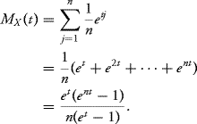
By differentiating with respect to t,

and

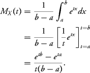
9.2 Suppose X has uniform distribution U[a, b] with a < b. Show that for every , we have

and M_X(0) = 1.

Solution: Clearly, M_X(0) = 1. For t ≠ 0,

9.3 Prove Proposition 9.17.

Solution: For every t, we have

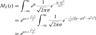
since

(density of a normal law).

9.4 Use the moment-generating function of X ~ N(μ, σ²) to prove that

Solution: From exercise 9.3, we get

and thus

Also,

and thus Then

9.5 Prove Proposition 9.18.

Solution: We have

for every .

9.6 Suppose that X admits a moment-generating function M_X. Prove that

and

(These are called the Chernoff bounds.)

Proof: One has

and

We can use Markov's inequality to conclude.

Problems without Solution

9.7 If X ~ Binom(n, p), use the moment generating function to get

9.8 Prove Proposition 9.8.

9.9 Show that

for any and θ [0, 2π], using generating functions.

9.10 Find the generating functions, both ordinary and moment-generating function, for the following discrete probability distributions.

9.11 Let X, Y be two random variables such that

and

9.12 Let X be a discrete r.v. with values in {0, 1, ..., n}. Let M_X denote its moment-generating function. Find in terms of M_X the moment-generating functions of

9.13 Use Proposition 9.19 to show that X ~ Γ(a, λ) and Y ~ Γ(b, λ) are two independent random variables, then

9.14 Suppose X has the density

where a > 0. This means that X follows a Pareto distribution (power law).

a. Show that M_X(t) =∞ for every .

b. Show that

if and only if a > n.

9.15 Suppose X ~ Poisson(a) with a > 0. Use exercise 6 to show that

9.16 Let X, Y be two random variables with moment-generating functions M_X and M_Y respectively. Show that X and Y have the same distribution if and only if

for any .

9.17 Let X ~ Exp(λ). Calculate EX³ and EX⁴. Give a general formula for EXⁿ.

9.18 Using the properties of the MGF, show that if X_i are i.i.d. Exp(λ) random variables, then

is distributed as a gamma random variable with parameters n and λ.

9.19 Prove the following facts about Laplace transform:

where Γ(n) denote the gamma function calculated at n.

9.20 Suppose f^* denotes the Laplace transform of the function f. Prove the following properties:

9.21 Suppose that X₁ ~ Exp(λ₁) and X₂ ~ Exp(λ₂) are independent. Given that the inverse laplace transform of the function is e^−cx and that the inverse Laplace transform is linear, calculate the p.d.f. of X₁ + X₂.

9.22 Repeat the problem above with three exponentially distributed random variables, that is, X_i ~ Exp(λ_i), i = 1, 2, 3. As a note, the distribution of a sum of n such independent exponentials is called the Erlang distribution and is heavily used in queuing theory.