Chapter Ten

Gaussian Random Vectors

10.1 Introduction/Purpose of the Chapter

Gaussian random variables and Gaussian random vectors (vectors whose components are jointly Gaussian, as defined in this chapter) play a central role in modeling real-life processes. Part of the reason for this is that noise like quantities encountered in many practical applications are reasonably modeled as Gaussian. Another reason is that Gaussian random variables and vectors turn out to be remarkably easy to work with (after an initial period of learning their features). Jointly Gaussian random variables are completely described by their means and covariances, which is part of the simplicity of working with them. Estimating these joint Gaussians means approximating only their means and covariances.

A third reason why Gaussian random variables and vectors are so important is that, in many cases, the performance measures we get for estimation and detection problems for the Gaussian case often bounds the performance for other random variables with the same means and covariances. For example, the minimum mean square estimator for Gaussian problems is the same as the linear least squares estimator for other problems with the same mean and covariance and, furthermore, has the same mean square performance. We will also find that this estimator has a simple expression as a linear function of the observations. Finally, we will find that the minimum mean square estimator for non-Gaussian problems always has a better performance than that for Gaussian problems with the same mean and covariance, but that the estimator is typically much more complex. The point of this example is that non-Gaussian problems are often more easily and more deeply understood if we first understand the corresponding Gaussian problem.

In this chapter, we develop the most important properties of Gaussian random variables and vectors, namely the moment-generating function, the moments, the joint densities, and the conditional probability densities.

10.2 Vignette/Historical Notes

The Gaussian distribution is named after Johann Carl Friedrich Gauss (30 April 1777–23 February 1855), one of the most famous mathematicians and physical scientists of the 18th century. Besides 301 probability and statistics, Gauss contributed significantly to many other fields, including number theory, analysis, differential geometry, geodesy, geophysics, electrostatics, astronomy, and optics.

Gauss work on a theory of the motion of planetoids disturbed by large planets, eventually published in 1809 as Theoria motus corporum coelestium in sectionibus conicis solem ambientum (Theory of motion of the celestial bodies moving in conic sections around the sun), contained an influential treatment of the method of least squares, a procedure which is used today in all sciences to minimize the impact of measurement error. Gauss proved the method under the assumption of normally distributed errors, a methodology that today is the first step in analysis of errors produced by very complex processes.

With the proper formulation of the Brownian motion (Wiener process) by Norbert Wiener in the 1950s the Gaussian process became mainstream for the theory of stochastic processes. The chaos theory developed in the 1970s owes a lot of gratitude to Gaussian processes to be able to produce useful formulas and bounds. Most of the machine learning theory uses assumptions about errors behaving like Gaussian processes. For all these reasons, learning about them is a crucial skill to be acquired by any aspiring student in probability.

10.3 Theory and Applications

10.3.1 The Basics

Let us first recall that a random variable follows the normal law N(μ, σ²) with σ > 0 if its density is given by

Before introducing the concept of Gaussian vector, let us list some properties of Gaussian random variables, which are already proven in the previous chapters of this book.

• The parameters μ and σ completely characterize the law of X.
• X ∼ N(μ, σ²) if and only if

• If X ∼ N(μ, σ²) and we denote μ_p = E(X − EX)^p = E(X − μ)^p, the p-central moment, then

• If X ∼ N(μ, σ²), then

• The sum of two independent normal random variables is normal; that is, if , and X, Y are independent, then

• The characteristic function of X ∼ N(μ, σ²) is

• The moment-generating function of X ∼ N(0, 1) is (see Proposition 9.16)

10.3.2 Equivalent Definitions of a Gaussian Vector

Let us now define the Gaussian vector.

The following two facts are immediate.

Proof: 1. Indeed, this follows from the definition by choosing α_i = 1 and α_j = 0 for every j ≠ i, j = 1, …, d.

2. It is a consequence of the definition of the Gaussian vector and of the Proposition 7.29. We mention that the assumption that X_i are independent is crucial. In this chapter, we will see examples showing that it is possible to have random vectors with each component Gaussian which are not Gaussian.

As we mention above, the mean and the variance characterize the law of a Gaussian random variable (one-dimensional). In the multidimensional case, the mean (which is a vector) and the covariance matrix will completely determine the law of a Gaussian vector.

Recall that if X = (X₁, …, X_d) is a random vector, then

and the covariance matrix of X, denoted by Λ_X = (Λ_X(i, j))_i,j=1,…,d, is defined by

for every i, j = 1, …, d.

Let us first remark that the mean and the covariance matrix of a Gaussian vector entirely characterize the first two moments (and thus the distribution) of every linear combination of the components of the vector. We recall the notation of a scalar product of two vectors:

if , and we denoted by x^T the transpose of the d × 1 matrix x.

Proof: It follows from Definition 10.1 that Y is a Gaussian r.v. (a linear combination of Gaussian random variables). It remains to compute its expectation and its variance. First

and

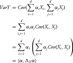
by noticing that the components of the vector are

Using Proposition 10.4, it is possible to obtain the characteristic function of a Gaussian vector.

Proof: By definition, we have

Using Proposition 10.4, we have that, by Eq. (10.1),

where Y = X, u . It suffices to note that

for every .

Proof: Let and define

For every we have

Suppose that X is a Gaussian vector. Since Λ_X is symmetric and positive definite, there exists such that

Let N₁ ∼ N(0, I_d). We apply Theorem 10.5 and the beginning of this proof. It follows that X and m + AN₁ have the same characteristic function and therefore the same law.

The converse of Theorem 10.7 is also true.

Proof: Let

and consider the linear combination

where (AN)_i is the component i of the vector , i = 1, …, d. Then, due to Proposition 10.4, we have

So every linear combination of the components of X is a Gaussian random variable, which means that X is a Gaussian vector.

By putting together the results in Theorems 10.5, 10.7, and 10.8, we obtain three alternative characterization of a Gaussian vector.

Proof: The implication 1 2 follows from Theorem 10.5. The implication 2 3 is a consequence of the proof of Theorem 10.7. The implication 3 1 has been showed in Theorem 10.8.

10.3.3 Uncorrelated Components and Independence

One of the most important properties of a Gaussian vector is the fact that its components are independent if and only if they are uncorrelated. One direction is always true for every random variable: If two random variables are independent, then they are uncorrelated. On the other hand, the converse is strongly related to the structure of the Gaussian vector, and it does not hold in general for other random variables. In Example 10.5 we show that that there exist Gaussian random variables (without the gaussian vector structure) which are uncorrelated but are not independent.

Proof: If X_i is independent by X_j, then clearly Cov(X_i, X_j) = 0, i ≠ j.

Suppose that Cov(X_i, X_j) = 0, i ≠ j. Denote by μ = EX and Λ_X = (λ_i,j)_i,j=1,…,d the mean vector and covariance matrix of the vector X. Since the individual covariances are zero, this matrix is a diagonal matrix and we have

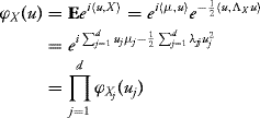
for every . We used the fact that for every j = 1, …, d, one has

Since the characteristic function of the vector is the product of individual characteristic functions, the components of the vector X are independent.

Solution: Indeed, it is easy to see that (U, V) is a Gaussian vector (every linear combination of its components is a linear combination of X and Y and (X, Y) is a Gaussian vector). Moreover,

and the independence is obtained from Theorem 10.12.

Solution: Let us first show that Y is a Gaussian vector. We note that

is a Gaussian vector with zero mean and covariance matrix I₄. Take . Then

and this is a Gaussian r.v. since X is a Gaussian vector. Moreover,

In the same way, we have

so Y₁, Y₂, Y₃ are independent random variables. In fact, the vector Y is a Gaussian vector with EY = 0 and covariance matrix

Solution: Since X − αY and Y are Gaussian random variables, it suffices to impose the condition

this implies

where we denoted with

the correlation coefficient between X and Y.

Solution: Let us show first that

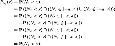
Indeed, by computing the cumulative distribution function of Y, we get for every

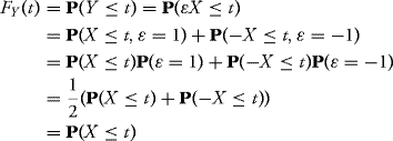
by using the fact that −X ∼ N(0, 1). So X, Y have the same law N(0, 1). Let us show that X, Y are uncorrelated. Indeed,

since Eε = 0. But it is easy to see that X and Y are not independent.

This example shows that it is possible to find two Gaussian uncorrelated r.v which are not independent. The reason why they are not independent is that the vector (X, Y) is not a Gaussian vector (see exercise 7.8).

A more general result can be stated as follows. The proof follows the arguments in the proof of Theorem 10.12.

10.3.4 The Density of a Gaussian Vector

Let X = (X₁, …, X_d) be a Gaussian vector with independent components. Assume that for every i = 1, …, d we have

In this case it is easy to write the density of the vector X. It is, from Corollary 7.23,

(10.3)

In the case of a standard normal vector X ∼ N(0, I_d), we have

When the components of X are not independent, we have the following.

Proof: From Theorem 10.7 we can write

where

We apply the change of variable formula (Theorem 7.24) to the function :

We have

We obtain

where f_N denotes the density of the vector N ∼ N(0, I_d). Since

and

we obtain the conclusion of the theorem.

However, in the case of degenerated Gaussian vectors, we have the property stated by the next proposition. We need to recall the notion of rank of a matrix. The rank of a matrix is the dimension of the vector space generated by its columns (or its rows). It is the largest possible dimension of a minor with determinant different from zero. A minor in a matrix can be constructed by eliminating any number of rows and columns. Obviously, if the d-dimensional matrix is invertible, then the rank of the matrix is d.

In the case of a Gaussian vector of dimension 2 (a Gaussian couple), we have the following:

Assume ρ² ≠ 1. Then the density of the vector X is

Proof: This follows from Theorem 10.4 since

10.3.5 Cochran's Theorem

Recall that if X ∼ N(0, 1), then , the gamma distribution with parameters and . This law is called the chi square distribution and is usually denoted by χ²(1), with 1 denoting one degree of freedom. More generally, if X₁, …, X_d are independent standard normal random variables, then

follows the law and this is called the chi square distribution with d degrees of freedom, denoted by χ²(d).

This situation can be extended to nonstandard normal random variables.

Recall that the modulus (or the Euclidean norm) of a d-dimensional vector is

We can now state the Cochran theorem.

Proof: Let

be an orthonormal basis of E_j. Then

The random vectors are independent of distribution , so the random vectors are independent. To finish, it suffices to remark that

for every j = 1, …, d.

Let us give an important application of the Cochran's theorem to Gaussian random vectors.

Proof: We set for every i = 1, …, n

Then Y_i are independent identically distributed N(0, 1). We also set

(by Vect(e) we mean the vector space of generated by the vector e). Then

The projections of Y = (Y₁, …, Y_n) on E, E^⊥ are independent and given by

and

We therefore have

and

which gives the conclusion.

10.3.6 Matrix Diagonalization and Gaussian Vectors

We start with some notion concerning eigenvalues and eigenvectors of a matrix.

Proof: Let λ be an eigenvalue of A. If u E_λ is a corresponding eigenvector, then for every , α ≠ 0 we have

so

(10.6)

which shows that E_λ is closed under multiplication with scalars.

If is another vector in E_λ, then

so

(10.7)

Relations (10.6) and (10.7) show that E_λ is a vector space in .

Proof: If λ is an eigenvalue for A, there exists u ≠ 0, such that Au = λu; therefore

This implies that the matrix A − λI_n is not invertible and thus det (A − λI_n) = 0 .

Conversely, if det (A − λI_n) = 0, then A − λI_n is not invertible so there exists nonidentically zero such that (A − λI_n)u = 0 .

Finally, if λ is an eigenvalue of A, then the set of associated eigenvectors are the vectors satisfying (A − λI_n)u = 0, which in fact is the definition of Ker(A − λI_n).

In the case when A is diagonalizable, every column of the matrix P represents an eigenvector for A and the diagonal matrix D contains on its diagonal the eigenvalues of A. Each column i is an eigenvector for the eigenvalue i on the diagonal of D.

The following results apply to any random vector and not only the Gaussian random vectors. We shall review the requirement of a covariance matrix.

Please note that u^TAu is a number, thus its sign is unique. Further, we always consider vectors in as matrices having dimension d × 1.

Proof: To prove this proposition, let us first remark that the covariance matrix is a square matrix. Next, the element on row i column j is

thus the matrix must be symmetric.

About the positive definiteness for any , we can construct the one-dimensional random variable: u^TX. Since this is a valid random variable, its variance must be non-negative. So let us calculate this variance:

Since the number squared is one-dimensional, and a one-dimensional number is equal to its transpose, we may write

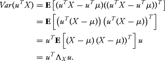
Thus, the condition that variance is non-negative translates into the condition that the covariance matrix is non-negative definite.

Checking that a square matrix is positive definite can be complicated. However, there is an easy way to check involving the eigenvalues of the matrix.

The following result is important because it can be applied to the covariance matrices.

The above result says that every symmetric positive definite matrix is diagonalizable in an orthonormal basis. That is, it can be transformed by elementary transformations into a diagonal matrix.

Proof: The proof follows by using Theorem 10.3.36. Since Λ_X is a symmetric matrix, it can be diagonalizable in an orthonormal basis. That is, there exists an orthogonal matrix B such that BΛ_XB^T is diagonal. The covariance of BX is BΛ_XB^T, so the components of BX are independent Gaussian random variables.

Exercises

Problems with Solution

10.1 Suppose

and define

Solution: Y is clearly a Gaussian vector since Y = AX with

where each component of Y is a linear combination of the original independent components Gaussian vector. To have the components of Y independent we need to impose the condition

But

Therefore if a + b = 0, the components Y₁, Y₂ are independent. Since

we will have in this case (a + b = 0)

10.2 Let X = (X₁, X₂, X₃) be a random vector in with density

Solution: Note that

where

To see this decomposition, please think about how the polynomial terms appear. It helps to note that the diagonal elements give the squares in a unique way and thus they are easy to recognize. For the off diagonal elements note that twice the element gives the coefficient (because the matrix is symmetric).

Once we write it in this form, we recognize the density of aGaussian vector X with zero mean and covariance matrix

Consequently,

To solve part (b), we need to impose that

and

To impose these conditions, we need to calculate the covariance matrix:

Thus we need to know how to invert a matrix or to use a software program to do so. Using R gives

The command “solve(M)” is the R command to find the inverse of the matrix M. We can now read the covariances between the original vector components X₁, X₂, X₃.

Now, using the matrix above and the formulas for the vector, the conditions are

V (X₁) is already 1. Using a = b and c = d from the first two equations, the later equations become

The first two equations are incompatible with a = 0, so we must have c = −e and either a = 1 or a = −1. Using this in the last equation gives e = 1. Thus the problem has more than one solution. Either of these vectors

will have the desired properties.

Finally, for part (c), since either one of these vectors is Gaussian by requiring that the covariance matrix is the identity, we found components which are mutually independent.

10.3 Let X, X, Z be independent standard normal random variables. Denote

and

(10.8)

Show that U and V are independent.

Solution: Define

Clearly, A is a Gaussian vector with and covariance matrix

the identity matrix. It follows that the vector

is also a Gaussian vector (every linear combination of its components is a linear combination of X, Y, Z). We will show that the first component is independent of all the other three. To prove this since the vector is Gaussian, it suffices to show that the first component is uncorrelated with the other three. We have

and in a similar way

Therefore the r.v. X + Y + Z is independent of X − Y, X − Z, and Y − Z respectively. By the associativity property of the independence, we have that X + Y + Z is independent of (X − Y, X − Z, Y − Z) and, thus, independent of V.

10.4 Let X₁, …, X_n be independent N(0, 1) distributed random variables. Let . Give a necessary and sufficient condition on the vector a in order to have X − a, X a and a, X independent.

Solution: The vector

is an (n + 1)-dimensional Gaussian vector and for every i = 1, …, n we obtain

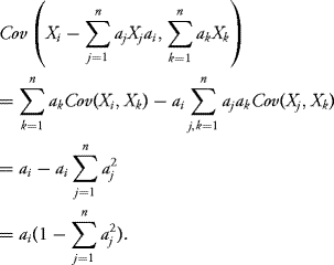
Therefore if we impose the condition

then all covariances between a, X and the other terms of the vector will be zero. This will accomplish what is needed in the problem.

10.5 Let X = (X₁, X₂, …, X_n) denote an n-dimensional random vector with independent components such that for every i = 1, …, n. Define

Solution: As a sum of independent normal random variables, is a normal random variable. Its parameters can be easily calculated as mean and variance . So

Note that the vector

is a Gaussian random vector. Indeed, every linear combination of its components is a linear combination of the components of X, so it is a Gaussian random variable. Therefore, and are independent if and only if they are uncorrelated; and after calculating the covariance, this is equivalent to

Hint for part (c): W_n is invariant by translation: W_n(X) = W_n(X + a) if X + a = (X₁ + a, . . ., X_n + a) for . Consider also Proposition 10.24.

10.6 Let (X, Y) be a Gaussian vector with mean 0 and covariance matrix

with ρ [− 1, 1]. What can be said about the random variables

Solution: Clearly, (X, Z) is a Gaussian vector as a linear transformation of a Gaussian vector. Since

we note that the r.v.'s X and Z are independent.

10.7 Suppose X ∼ N(0, 1). Prove that for every x > 0 the following inequalities hold:

Solution: Consider the following functions defined on (0, ∞):

and

We need to show that

for every x > 0, where F is the c.d.f. of an N(0, 1) distributed random variable.

Since the normal c.d.f. does not have a closed form, we look at the derivatives of these functions. We need to check that for x > 0:

where is the standard normal density. Therefore, integrating the respective positive functions on (0, ∞), we obtain

and

Problems without Solution

10.8 Suppose

Show that XY has the same law as

Hint: Use the polarization formula

10.9 Prove the expression of the density function of the noncentral chi square distribution (10.5).

10.10 Let (X, Y) be a two-dimensional Gaussian vector with zero expectation and I₂ covariance matrix. Compute

10.11 Let X, Y be two independent N(0, 1) distributed random variables. Define

10.12 Let X₁, …, X_n be i.i.d. N(0, 1) random variables. Define

Compare and calculate EU and EV.

10.13 Let with

10.14 Suppose X ∼ N(0, Λ) where

Let

10.15 Let X = (X₁, X₂, X₃) be a Gaussian vector with law N₃(m, C) with density

where

10.16 Let (X, Y) be a normal random vector such that X and Y are standard normal N(0, 1). Suppose that Cov(X, Y) = ρ. Let and put

10.17 Let (X, Y, Z) be a Gaussian vector with mean (1, 2, 3) and covariance matrix

Set

10.18 If X is a standard normal random variable N(0, 1), let ϕ denote its characteristic function and F its c.d.f. For every p ≥ 1 integer, denote the p moment with

Let (Y_n , n ≥ 1) be a sequence of independent r.v. with identical distribution N(0, 1). For every k ≥ 1 and n ≥ 1 integers, let

10.19 Let X₁, X₂, and X₃ be three i.i.d. random variables where their distribution has zero mean and variance σ² > 0. Denote

10.20 If X ∼ N(0, 1) and Y ∼ χ²(n, 1) and X, Y are independent, show that

has a Student t distribution (t_n) with n degrees of freedom. Specifically, show that the probability density function of Z is given by

10.21 Assume X and Y are two independent N(0, 1) random variables. Find the law of

Hint: We know (how to prove) that X + Y and X − Y are independent and each has N(0, 2) distribution. Then, once we show that

is χ²(1) distributed, we will obtain

which follows a Student distribution with one degree of freedom (see exercise 20).

10.22 Consider the matrix

10.23 Consider the matrix

10.24 Let the matrix Σ be defined as

Check that the matrix is symmetric and positive definite. Find its eigenvalues and the associated eigenvectors. Now, let X be a Gaussian random vector with covariance matrix Σ and zero mean. Find a linear transformation that transforms X in a Gaussian vector with independent components.