As a first step, we would like to visualize the average period return by factor quantile. We can use the built-in function mean_return_by_quantile from the performance and plot_quantile_returns_bar from the plotting modules:

from alphalens.performance import mean_return_by_quantile
from alphalens.plotting import plot_quantile_returns_bar
mean_return_by_q, std_err = mean_return_by_quantile(alphalens_data)
plot_quantile_returns_bar(mean_return_by_q);

The result is a bar chart that breaks down the mean of the forward returns for the four different holding periods based on the quintile of the factor signal. As you can see, the bottom quintiles yielded markedly more negative results than the top quintiles, except for the longest holding period:

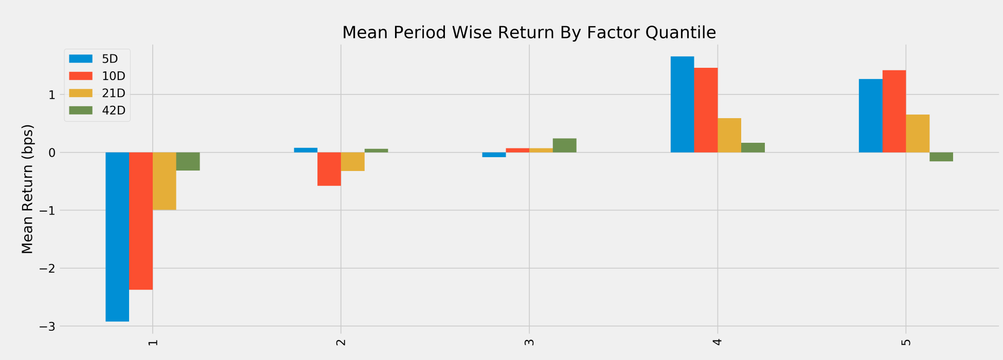
The 10D holding period provides slightly better results for the first and fourth quartiles. We would also like to see the performance over time of investments driven by each of the signal quintiles. We will calculate daily, as opposed to average returns for the 5D holding period, and alphalens will adjust the period returns to account for the mismatch between daily signals and a longer holding period (for details, see docs):

from alphalens.plotting import plot_cumulative_returns_by_quantile
mean_return_by_q_daily, std_err =     
     mean_return_by_quantile(alphalens_data, by_date=True)
plot_cumulative_returns_by_quantile(mean_return_by_q_daily['5D'], 
     period='5D');

The resulting line plot shows that, for most of this three-year period, the top two quintiles significantly outperformed the bottom two quintiles. However, as suggested by the previous plot, signals by the fourth quintile produced a better performance than those by the top quintile:

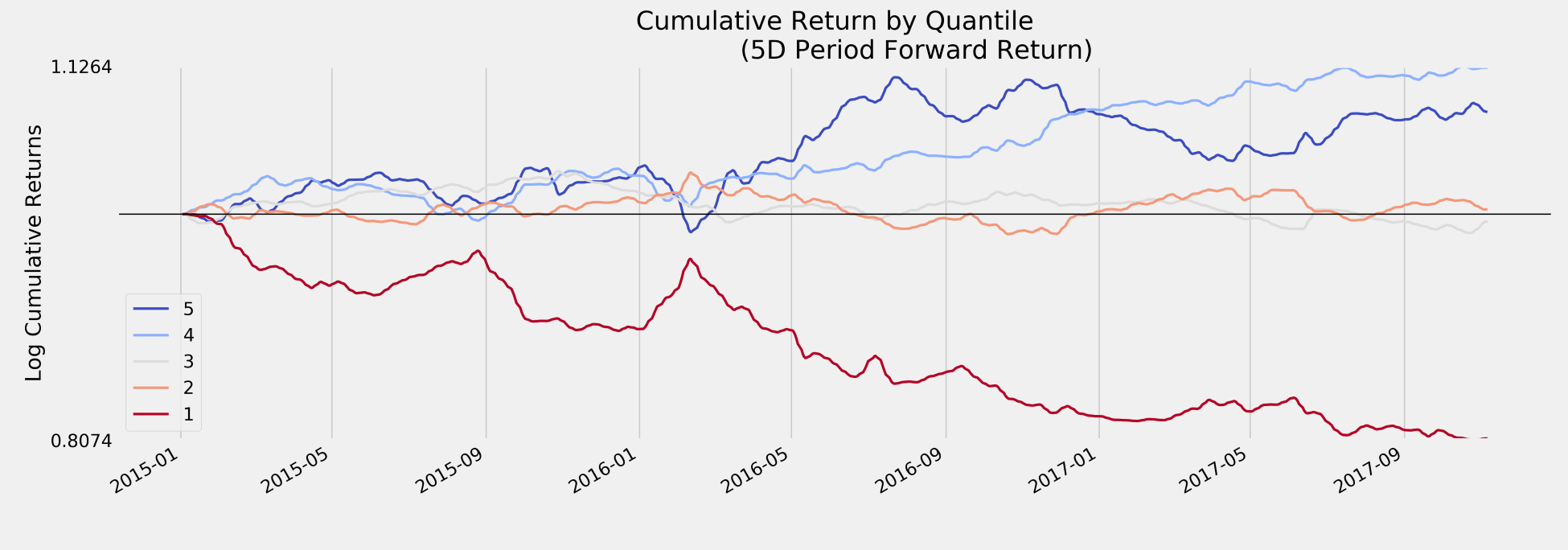
A factor that is useful for a trading strategy shows the preceding pattern where cumulative returns develop along clearly distinct paths because this allows for a long-short strategy with lower capital requirements and correspondingly lower exposure to the overall market.

However, we also need to take the dispersion of period returns into account rather than just the averages. To this end, we can rely on the built-in plot_quantile_returns_violin:

from alphalens.plotting import plot_quantile_returns_violin
plot_quantile_returns_violin(mean_return_by_q_daily);

This distributional plot highlights that the range of daily returns is fairly wide and, despite different means, the separation of the distributions is very limited so that, on any given day, the differences in performance between the different quintiles may be rather limited:

While we focus on the evaluation of a single alpha factor, we are simplifying things by ignoring practical issues related to trade execution that we will relax when we address proper backtesting in the next chapter. Some of these include:

• The transaction costs of trading
• Slippage, the difference between the price at decision and trade execution, for example, due to the market impact