Regression trees make predictions based on the mean outcome value for the training samples assigned to a given node and typically rely on the mean-squared error to select optimal rules during recursive binary splitting.

Given a training set, the algorithm iterates over the predictors, X₁, X₂, ..., X_p, and possible cutpoints, s₁, s₁, ..., s_N, to find an optimal combination. The optimal rule splits the feature space into two regions, {X|X_i < s_j} and {X|X_i > s_j}, with values for the X_i feature either below or above the s_j threshold so that predictions based on the training subsets maximize the reduction of the squared residuals relative to the current node.

Let's start with a simplified example to facilitate visualization and only use two months of lagged returns to predict the following month, in the vein of an AR(2) model from the last chapter:

Using sklearn, configuring and training a regression tree is very straightforward:

from sklearn.tree import DecisionTreeRegressor

# configure regression tree
regression_tree = DecisionTreeRegressor(criterion='mse', # default
                                        max_depth=4,     # up to 4 splits
                                        random_state=42)
# Create training data
y = data.returns
X = data.drop('returns', axis=1)
X2 = X.loc[:, ['t-1', 't-2']]

# fit model
regression_tree.fit(X=X2, y=y)

# fit OLS model
ols_model = sm.OLS(endog=y, exog=sm.add_constant(X2)).fit()

The OLS summary and a visualization of the first two levels of the decision tree reveal the striking differences between the model. The OLS model provides three parameters for the intercepts and the two features in line with the linear assumption this model makes about the f function.

In contrast, the regression tree chart displays, for each node of the first two levels, the feature and threshold used to split the data (note that features can be used repeatedly), as well as the current value of the mean-squared error (MSE), the number of samples, and predicted value based on these training samples:

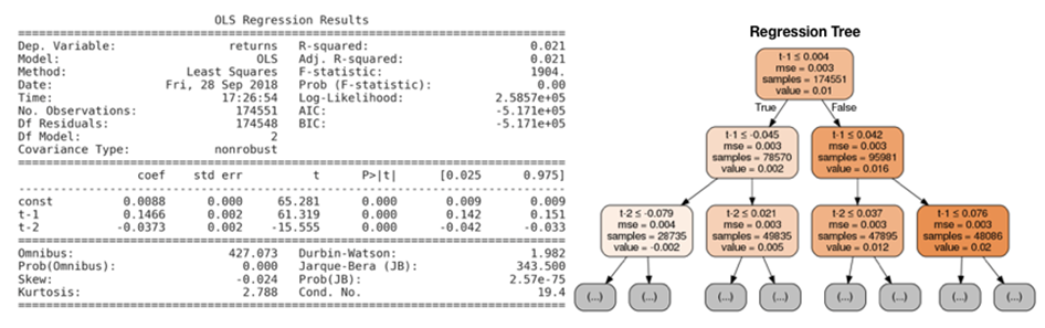
The tree chart also highlights the uneven distribution of samples across the nodes as the numbers vary between 28,000 and 49,000 samples after only two splits.

To further illustrate the different assumptions about the functional form of the relationships between the input variables and the output, we can visualize current return predictions as a function of the feature space, that is, as a function of the range of values for the lagged returns. The following figure shows the current period return as a function of returns one and two periods ago for linear regression and the regression tree:

The linear-regression model result on the right side underlines the linearity of the relationship between lagged and current returns, whereas the regression tree chart on the left illustrates the non-linear relationship encoded in the recursive partitioning of the feature space.