We have a salesman who must travel between n cities. He doesn't care about which order this happens in, nor which city he visits first or last. His only concern is that he visits each city only once and finishes at home, where he started.
Now, each of those connections has one or more weights associated with it, which we will call the cost.
Our salesman has a boss as we met in Chapter 1, Machine Learning Basics, so his marching orders are to keep the cost and distance he travels as low as possible.
How does this apply to me in real life? you may ask. This problem actually has several applications in real life such as
- The design and creation of circuit boards for your computer. With millions of transistors, the circuit board needs to be drilled and created precisely.
- It also appears as a subproblem in DNA sequencing, which has become a big part of machine learning for many people.
For those that have taken up or are familiar with graph theory, you hopefully remember the undirected weighted graph. That is exactly what we are dealing with here. The cities are vertices, the paths are edges, and the path distance is the edge weight. Never thought you'd use that knowledge again, did you? In essence, we have a minimization problem of starting and finishing at a specific vertex after having visited every other vertex just once. We may, in fact, end up with a complete graph when we are done, where each pair of vertices is connected by an edge.
Next, we must talk about asymmetry and symmetry, because this problem may end up being either. What do we mean exactly? Well, we have either an asymmetric traveling salesman problem or a symmetric traveling salesman problem. It all depends upon the distance between two cities. If the distances are the same in each direction, we have a symmetric traveling salesman problem, and the symmetry helps us have the possible solutions. If the paths do not exist in both directions, or if the distances are different, we have a directed graph. Here is a diagram showing the preceding description:

The traveling salesman problem can be symmetric or asymmetric. In this chapter, we are going to take you through the wonderful land of genetic algorithms. Let's start with an incredibly oversimplistic description of what's going to happen.
In the biology world, when we want to create a new genotype, we take a little bit from parent A and the rest from parent B. This is called crossover mutation, if you are updating your buzzword-compliant checklist! After this happens, these genotypes are perturbed, or altered, ever so slightly. This is called mutation (update that buzzword compliant list again), and this is how genetic material is created.
Next, we delete the original generation, replaced by the new one, and each genotype is tested. The newer genotypes, being the better part of their previous components, will now be skewed towards higher fitness; on an average, this generation should score higher than its predecessor.
This process continues for many generations, and over time, the average fitness of the population will evolve and increase. This doesn't always work, as in real life, but generally speaking, it does.
With a seminar of genetic algorithmic programming behind us, let's dive into our application.
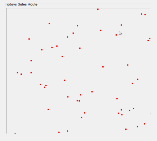
Here's what our sample application looks like. It is based on the Accord.NET framework. After we've defined the number of houses we need to visit, we simply click on the Generate button:

In our test application, we can change the number of houses that we want to visit very easily, as shown in the highlighted area.
We could have a very simple problem space or a more complicated one. Here is an example of a very simple problem space:

And here is an example of a more complicated problem space:
We also have three different types of selection methods for our algorithm to work with, namely Elite, Rank, and Roulette:

- Elite: Specifies the number of best chromosomes to work within the next generation.
- Roulette: Selects chromosomes based on their rank (fitness value).
- Rank: Selects chromosomes based on their rank (fitness value). This differs from the Roulette selection method in that the wheel and sector sizes are different within the calculation.
Finally, we choose the total number of iterations we want our algorithm to use. We select the Calculate Route button, and, assuming all goes well, we'll end up with our map looking similar to this:

Let's take a look at what happens when we select the number of cities we want and then click on the Generate button:
        private void GenerateMap( )
         {
             Random rand = new Random( (int) DateTime.Now.Ticks );

             // create coordinates array
             map = new double[citiesCount, 2];

             for ( int i = 0; i < citiesCount; i++ )
             {
                 map[i, 0] = rand.Next( 1001 );
                 map[i, 1] = rand.Next( 1001 );
             }

             // set the map
             mapControl.UpdateDataSeries( "map", map );
             // erase path if it is
             mapControl.UpdateDataSeries( "path", null );
         }
The first thing that we do is initialize our random number generator and seed it. Next, we get the total number of cities that the user specified, and then create a new array from that. Finally, we plot each point and update our map. The map is a chart control from Accord.NET that will take care of a lot of visual plotting for us.
With that done, we are ready to calculate our route and (hopefully) solve our problem.
Next, let's see what our main search solution looks like:
            Neuron.RandRange = new Range( 0, 1000 );
             DistanceNetwork network = new DistanceNetwork( 2, neurons );
             ElasticNetworkLearning    trainer = new ElasticNetworkLearning(
 network );
             double    fixedLearningRate = learningRate / 20;
             double    driftingLearningRate = fixedLearningRate * 19;
             double[,] path = new double[neurons + 1, 2];
             double[] input = new double[2];
             int i = 0;

             while ( !needToStop )
             {
                 trainer.LearningRate = driftingLearningRate * ( iterations - i ) / iterations + fixedLearningRate;
                 trainer.LearningRadius = learningRadius * ( iterations - i ) / iterations;

                 int currentCity = rand.Next( citiesCount );
                 input[0] = map[currentCity, 0];
                 input[1] = map[currentCity, 1];

                 trainer.Run( input );

                 for ( int j = 0; j < neurons; j++ )
                 {
                     path[j, 0] = network.Layers[0].Neurons[j].Weights[0];
                     path[j, 1] = network.Layers[0].Neurons[j].Weights[1];
                 }
                 path[neurons, 0] = network.Layers[0].Neurons[0].Weights[0];
                 path[neurons, 1] = network.Layers[0].Neurons[0].Weights[1];

                 chart?.UpdateDataSeries( "path", path );
                 i++;

                 SetText( currentIterationBox, i.ToString( ) );

                 if ( i >= iterations )
                     break;
            }
Let's try and break all that down into more usable chunks for you. The first thing we do is determine the selection method that we'll use to rank our chromosomes:
// create fitness function
 TSPFitnessFunction fitnessFunction = new TSPFitnessFunction( map );
 // create population
 Population population = new Population( populationSize,
     ( greedyCrossover ) ? new TSPChromosome( map ) : new PermutationChromosome( citiesCount ),
     fitnessFunction,
     ( selectionMethod == 0 ) ? (ISelectionMethod) new EliteSelection( ) :
     ( selectionMethod == 1 ) ? (ISelectionMethod) new RankSelection( ) :
     (ISelectionMethod) new RouletteWheelSelection( ));
I want to take this opportunity to point out the TSPChromosome you see here. This object is based on a short-array chromosome (one that is an array of unsigned short values ranging from 2 to 65,536. There are two specific features:
- All genes are unique within the chromosome, meaning there are no two genes with the same value
- The maximum value of each gene is equal to the chromosome length minus 1
Next, we must create the path variable for us to fill in with our data points:
double[,] path = new double[citiesCount + 1, 2];
After this is complete, we can enter our while loop and begin our processing. To do that, we will process a single generation by running a single epoch. You can think of an epoch as an iteration:
                // run one epoch of genetic algorithm
                 RILogManager.Default?.SendDebug("Running Epoch " + i);
                 population.RunEpoch( );
We then get the best values from that effort:
ushort[] bestValue = ((PermutationChromosome) population.BestChromosome).Value;
We update and create our path between each city:
for ( int j = 0; j < citiesCount; j++ )
                 {
                     path[j, 0] = map[bestValue[j], 0];
                     path[j, 1] = map[bestValue[j], 1];
                 }
                 path[citiesCount, 0] = map[bestValue[0], 0];
                 path[citiesCount, 1] = map[bestValue[0], 1];
And we supply that value to our chart control:
mapControl.UpdateDataSeries( "path", path );
Let's see some examples of what our route might look like based on the selection method that we choose.
The Elite selection:

The Rank selection:

The difference between this and the Roulette selection method is in the wheel and its sector size calculation methods. The size of the wheel equals size * (size +1) / 2, where size is the size of the current population. The worst chromosome has its sector size equal to 1, the next has a size of 2, and so on.
The Roulette selection:

This algorithm selects chromosomes of the new generation according to their fitness values. The higher the value, the greater the chances of it becoming a member of the new generation.
What you will notice as you generate your routes is that the Elite method finds its solution right away. The Rank method continues refining its route throughout the iterations, and the Roulette method refines its routes even more.
To illustrate what I mean, define a huge load for your salesman today. Let's say he has 200 houses to visit, as we need to sell a lot of encyclopedias today. This is where the beauty of our algorithm shines. It's easy to create the optimal map and route if we are dealing with five houses. But if we are dealing with 200 houses, not so much!

Now that we've solved our problem, let's see if we can apply what we learned from our earlier chapter about self-organizing maps (SOM) here to approach this problem from a different angle. If you recall, back in Chapter 6, Color Blending – Self-Organizing Maps and Elastic Neural Networks, we discussed SOM in general. So we'll preclude the academia from happening here! We're going to use a technique called Elastic Network Training, which is a great unsupervised approach to such a problem as we have here.

Let's first talk briefly about what an Elastic Map is. Elastic Maps provide a tool for creating nonlinear dimensionality reduction. They are a system of elastic springs in our data space that approximate a low-dimensional manifold. With this capability, we can go from completely unstructured clustering (no elasticity) to a closer linear principal components analysis manifold for high bending/low stretching of the springs. You'll see when using our sample application that the lines are not necessarily as rigid as they were in our previous solution. And in many cases, they may not even get into the center of the city we are visiting (the line generates off the center) but approach only the outskirts of the city limits, as in the preceding example!
Once again, we'll be dealing with neurons, one of my favorite objects of all. This time we'll have a bit more control though, by being able to specify our learning rate and radius. As with our previous example, we'll be able to specify the total number of cities our salesman must visit today. Let's go easier on him this time though!
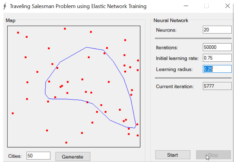
To start, we'll visit 50 cities and use a learning rate of 0.3 and radius of 0.75. Finally, we will run for 50,000 iterations (don't worry; this will go fast). Our output will look like this:

Now, what happens if we change our radius to a different value, say, 0.25? Note how our angles between some cities become more pronounced:

Next, let's change our learning rate from 0.3 to 0.75:

Even though our route looks very similar in the end, there is one important difference. In the previous example, the route path for our salesman was not drawn until all the iterations were complete. By raising the learning rate, the route gets drawn several times before the perfect route is complete. Here are some images showing the progression:

Here we are at iteration 5777 of our solution:
This shows how our solution looks at iteration 44636:

This one shows how our solution looks at iteration 34299:

Now, let's look into a small bit of code to see how our search solution differs this time:
            // create fitness function
             TSPFitnessFunction fitnessFunction = new TSPFitnessFunction( map );
             // create population
             Population population = new Population( populationSize,
                 ( greedyCrossover ) ? new TSPChromosome( map ) : new PermutationChromosome( citiesCount ),
                 fitnessFunction, ( selectionMethod == 0 ) ? new EliteSelection( )
                 : ( selectionMethod == 1 ) ? new RankSelection( ) :
                 (ISelectionMethod) new RouletteWheelSelection( ));
             // iterations
             int i = 1;

             // path
             double[,] path = new double[citiesCount + 1, 2];

             // loop
             while ( !needToStop )
             {
                 // run one epoch of genetic algorithm
                 RILogManager.Default?.SendDebug("Running Epoch " + i);
                 population.RunEpoch( );

                 // display current path
                 ushort[] bestValue = ((PermutationChromosome) population.BestChromosome).Value;

                 for ( int j = 0; j < citiesCount; j++ )
                 {
                     path[j, 0] = map[bestValue[j], 0];
                     path[j, 1] = map[bestValue[j], 1];
                 }
                 path[citiesCount, 0] = map[bestValue[0], 0];
                 path[citiesCount, 1] = map[bestValue[0], 1];

                 mapControl.UpdateDataSeries( "path", path );
                 // set current iteration's info
                 SetText( currentIterationBox, i.ToString( ) );
                 SetText( pathLengthBox, fitnessFunction.PathLength( population.BestChromosome ).ToString( ) );

                 // increase current iteration
                 i++;

                 //
                 if ( ( iterations != 0 ) && ( i > iterations ) )
                     break;
             }
The first thing you see that we've done is creating a DistanceNetwork object. This object contains only a single DistanceLayer, which is a single layer of distance neurons. A distance neuron computes its output as the distance between its weights and inputs—the sum of absolute differences between the weight values and input values. All of this together makes up our SOM and, more importantly, our Elastic Network.
Next, we have to initialize our network with some random weights. We will do this by creating a uniform continuous distribution for each neuron. A uniform continuous distribution, or rectangular distribution, is a symmetric probability distribution such that, for each member of the family, all intervals of the same length on the distribution's support have the same probability. You will usually see this written out as U(a, b), with parameters a and b being the minimum and maximum values respectively.
foreach (var neuron in network.Layers.SelectMany(layer => layer?.Neurons).Where(neuron => neuron != null))
 {
                 neuron.RandGenerator = new UniformContinuousDistribution(new Range(0, 1000));
 }
Next, we create our elastic learner object, which allows us to train our distance network:
ElasticNetworkLearning trainer = new ElasticNetworkLearning(network);
Here's what the ElasticNetworkLearning constructor looks like internally:

Now we calculate our learning rate and radius:
            double fixedLearningRate = learningRate / 20;
             double driftingLearningRate = fixedLearningRate * 19;
Finally, we are in our central processing loop, where we will remain until told to stop:
while (!needToStop)
             {
                 // update learning speed & radius
                 trainer.LearningRate = driftingLearningRate * (iterations - i) / iterations + fixedLearningRate;
                 trainer.LearningRadius = learningRadius * (iterations - i) / iterations;

                 // set network input
                 int currentCity = rand.Next(citiesCount);
                 input[0] = map[currentCity, 0];
                 input[1] = map[currentCity, 1];

                 // run one training iteration
                 trainer.Run(input);

                 // show current path
                 for (int j = 0; j < neurons; j++)
                 {
                     path[j, 0] = network.Layers[0].Neurons[j].Weights[0];
                     path[j, 1] = network.Layers[0].Neurons[j].Weights[1];
                 }
                 path[neurons, 0] = network.Layers[0].Neurons[0].Weights[0];
                 path[neurons, 1] = network.Layers[0].Neurons[0].Weights[1];

                 chart.UpdateDataSeries("path", path);

                 i++;

                 SetText(currentIterationBox, i.ToString());

                 if (i >= iterations)
                     break;
             }
In the preceding loop, the trainer is running one epoch (iteration) per loop increment. Here's what the trainer.Run function looks like, so you can see what's happening. Basically, the method finds the winning neuron (the one that has the weights with values closest to the specified input vector). It then updates its weights as well as the weights of the neighboring neurons:
public double Run( double[] input )
         {
             double error = 0.0;

             // compute the network
             network.Compute( input );
             int winner = network.GetWinner( );

             // get layer of the network
             Layer layer = network.Layers[0];

             // walk through all neurons of the layer
             for ( int j = 0; j < layer.Neurons.Length; j++ )
             {
                 Neuron neuron = layer.Neurons[j];

                 // update factor
                 double factor = Math.Exp( -distance[Math.Abs( j - winner )] / squaredRadius2 );

                 // update weights of the neuron
                 for ( int i = 0; i < neuron.Weights.Length; i++ )
                 {
                     // calculate the error
                     double e = ( input[i] - neuron.Weights[i] ) * factor;
                     error += Math.Abs( e );
                     // update weight
                     neuron.Weights[i] += e * learningRate;
                 }
             }
             return error;
         }
The two main functions of this method that we will look deeper into are computing the network and obtaining the winner (highlighted items).
How do we compute the network? Basically, we work ourselves down through the distance layer and into each neuron in order to update the weights correctly, similar to what you see here:
public virtual double[] Compute( double[] input )
         {
             // local variable to avoid mutlithread conflicts
             double[] output = input;

             // compute each layer
             for ( int i = 0; i < layers.Length; i++ )
             {
                 output = layers[i].Compute( output );
             }

             // assign output property as well (works correctly for single threaded usage)
             this.output = output;

             return output;
         }
Finally, we need to compute the winner, the neuron with the minimum weight and therefore the minimum distance:
public int GetWinner( )
         {
             // find the MIN value
             double min = output[0];
             int    minIndex = 0;

             for ( int i = 1; i < output.Length; i++ )
             {
                 if ( output[i] < min )
                 {
                     // found new MIN value
                     min = output[i];
                     minIndex = i;
                 }
             }

             return minIndex;
         }
Let's talk briefly about the parameters you can enter on the screen.