Using the linear algebra facilities of the Dlib library (or any other library, for that matter), we can implement anomaly detection with the multivariate Gaussian distribution approach. The following example shows how to implement this approach with the Dlib linear algebra routines:

void multivariateGaussianDist(const Matrix& normal,
                               const Matrix& test) {
     // assume that rows are samples and columns are features
     
     // calculate per feature mean
     dlib::matrix<double> mu(1, normal.nc());
     dlib::set_all_elements(mu, 0);
     
     for (long c = 0; c < normal.nc(); ++c) {
         auto col_mean = dlib::mean(dlib::colm(normal, c));
         dlib::set_colm(mu, c) = col_mean;
     }
     
     // calculate covariance matrix
     dlib::matrix<double> cov(normal.nc(), normal.nc());
     dlib::set_all_elements(cov, 0);
     for (long r = 0; r < normal.nr(); ++r) {
         auto row = dlib::rowm(normal, r);
         cov += dlib::trans(row - mu) * (row - mu);
     }
     cov *= 1.0 / normal.nr();
     double cov_det = dlib::det(cov); // matrix determinant
     dlib::matrix<double> cov_inv = dlib::inv(cov); // inverse matrix
     
     // define probability function
     auto first_part =
     1. / std::pow(2. * M_PI, normal.nc() / 2.) / std::sqrt(cov_det);
     
     auto prob = [&](const dlib::matrix<double>& sample) {
         dlib::matrix<double> s = sample - mu;
         dlib::matrix<double> exp_val_m = s * (cov_inv * dlib::trans(s));
         double exp_val = -0.5 * exp_val_m(0, 0);
         double p = first_part * std::exp(exp_val);
         return p;
     };
     
     // change this parameter to see the decision boundary
     double prob_threshold = 0.001;
     
     auto detect = [&](auto samples) {
         for (long r = 0; r < samples.nr(); ++r) {
             auto row = dlib::rowm(samples, r);
             auto p = prob(row);
             if (p >= prob_threshold) {
                 // Do something with anomalies
             } else {
                 // Do something with normal
             }
         }
     };
     
     detect(normal);
     detect(test);
 }

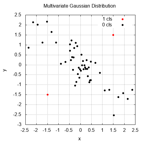
The idea of this approach is to define a function that returns the probability of appearing, given a sample in a dataset. To implement such a function, we calculate the statistical characteristics of the training dataset. In the first step, we calculate the mean values of each feature and store them into the one-dimensional matrix. Then, we calculate the covariance matrix for the training samples using the formula for the correlation matrix that was given in the prior theoretical section named Density estimation approach for anomaly detection. Next, we determine the correlation matrix determinant and inverse version. We define a lambda function named prob to calculate the probability of a single sample using the formula for the probability calculation that was given in the Density estimation approach for anomaly detection section. We also define a probability threshold to separate anomalies.

Then, we iterate over all the examples (including the training and testing datasets) to find out how the algorithm separates regular samples from anomalies. In the following graph, we can see the result of this separation. The dots marked with a lighter color are anomalies: