Isolation forest algorithms can be easily implemented in pure C++ because its logic is pretty straightforward. Also, there are no implementations of this algorithm in popular C++ libraries. Let's assume that our implementation will only be used with two-dimensional data. We are going to detect anomalies in a range of samples where each sample contains the same number of features.
Because our dataset is large enough, we can define a wrapper for the actual data container. This allows us to reduce the number of copy operations we perform on the actual data:
 using DataType = double;
 template <size_t Cols>
 using Sample = std::array<DataType, Cols>;
 template <size_t Cols>
 using Dataset = std::vector<Sample<Cols>>;
 ...
 template <size_t Cols>
 struct DatasetRange {
     DatasetRange(std::vector<size_t>&& indices, const Dataset<Cols>*
     dataset)
         : indices(std::move(indices)), dataset(dataset) {}
     size_t size() const { return indices.size(); }
     DataType at(size_t row, size_t col) const {
         return (*dataset)[indices[row]][col];
     }

     std::vector<size_t> indices;
     const Dataset<Cols>* dataset;
 };
The DatasetRange type holds a reference to the vector of Sample type objects and to the container of indices that point to the samples in the dataset. These indices define the exact dataset objects that this DatasetRange object points to.
Next, we define the elements of the isolation tree, with the first one being the Node type:
struct Node {
     Node() {}
     Node(const Node&) = delete;
     Node& operator=(const Node&) = delete;
     Node(std::unique_ptr<Node> left,
          std::unique_ptr<Node> right,
          size_t split_col,
          DataType split_value)
         : left(std::move(left)),
           right(std::move(right)),
           split_col(split_col),
           split_value(split_value) {}
     Node(size_t size) : size(size), is_external(true) {}

     std::unique_ptr<Node> left;
     std::unique_ptr<Node> right;
     size_t split_col{0};
     DataType split_value{0};
     size_t size{0};
     bool is_external{false};
 };
This type is a regular tree node structure. The following members are specific to the isolation tree algorithm:
- split_col: This is the index of the feature column where the algorithm caused a split.
- split_value: This is the value of the feature where the algorithm caused a split.
- size: This is the number of underlying items for the node.
- is_external: This is the flag that indicates whether the node is a leaf.
Taking the Node type as a basis, we can define the procedure of building an isolation tree. We aggregate this procedure with the auxiliary IsolationTree type. Because the current algorithm is based on random splits, the auxiliary data is the random engine object.
We only need to initialize this object once, and then it will be shared among all tree type objects. This approach allows us to make the results of the algorithm reproducible in the case of constant seeding. Furthermore, it makes debugging the randomized algorithm much simpler:
 template <size_t Cols>
 class IsolationTree {
 public:
     using Data = DatasetRange<Cols>;

     IsolationTree(const IsolationTree&) = delete;
     IsolationTree& operator=(const IsolationTree&) = delete;
     IsolationTree(std::mt19937* rand_engine, Data data, size_t hlim)
         : rand_engine(rand_engine) {
         root = MakeIsolationTree(data, 0, hlim);
     }
     IsolationTree(IsolationTree&& tree) {
         rand_engine = std::move(tree.rand_engine);
         root = td::move(tree.root);
     }

     double PathLength(const Sample<Cols>& sample) {
         return PathLength(sample, root.get(), 0);
     }

 private:
     std::unique_ptr<Node> MakeIsolationTree(const Data& data,
                                             size_t height,
                                             size_t hlim);

     double PathLength(const Sample<Cols>& sample,
                       const Node* node,
                       double height);

 private:
     std::mt19937* rand_engine;
     std::unique_ptr<Node> root;
 };
Next, we'll do the most critical work in the MakeIsolationTree() method, which is used in the constructor to initialize the root data member:
std::unique_ptr<Node> MakeIsolationTree(const Data& data,
                                         size_t height,
                                         size_t hlim) {
     auto len = data.size();
     if (height >= hlim || len <= 1) {
         return std::make_unique<Node>(len);
     } else {
         std::uniform_int_distribution<size_t> cols_dist(0, Cols - 1);
         auto rand_col = cols_dist(*rand_engine);

         std::unordered_set<DataType> values;
         for (size_t i = 0; i < len; ++i) {
             auto value = data.at(i, rand_col);
             values.insert(value);
         }

         auto min_max = std::minmax_element(values.begin(), values.end());
         std::uniform_real_distribution<DataType>
            value_dist(*min_max.first, *min_max.second);
         auto split_value = value_dist(*rand_engine);

         std::vector<size_t> indices_left;
         std::vector<size_t> indices_right;
         for (size_t i = 0; i < len; ++i) {
             auto value = data.at(i, rand_col);
             if (value < split_value) {
                 indices_left.push_back(data.indices[i]);
             } else {
                 indices_right.push_back(data.indices[i]);
             }
         }

         return std::make_unique<Node>(
             MakeIsolationTree(Data{std::move(indices_left), data.dataset},
                           height + 1, hlim),
             MakeIsolationTree(Data{std::move(indices_right),
                           data.dataset}, height + 1, hlim),
             rand_col,
             split_value);
     }
 }
Initially, we checked the termination conditions to stop the splitting process. If we meet them, we return a new node marked as an external leaf. Otherwise, we start splitting the passed data range. For splitting, we randomly select the feature column and determine the unique values of the selected feature. Then, we randomly select a value from an interval between the max and the min values among the feature values from all the samples. After we make these random selections, we compare the values of the selected splitting feature to all the samples from the input data range and put their indices into two lists. One list is for values higher than the splitting values, while another list is for values that are lower than them. Then, we return a new tree node initialized with references to the left and right nodes, which are initialized with recursive calls to the MakeIsolationTree() method.
Another vital method of the IsolationTree type is the PathLength() method. We use it for anomaly score calculations. It takes the sample as an input parameter and returns the amortized path length to the corresponding tree leaf from the root node:
double PathLength(const Sample<Cols>& sample,
                   const Node* node,
                   double height) {
     assert(node != nullptr);
     if (node->is_external) {
         return height + CalcC(node->size);
     } else {
         auto col = node->split_col;
         if (sample[col] < node->split_value) {
             return PathLength(sample, node->left.get(), height + 1);
         } else {
             return PathLength(sample, node->right.get(), height + 1);
         }
     }
 }
The PathLength() method finds the leaf node during tree traversal based on sample feature values. These values are used to select a tree traversal direction based on the current node splitting values. During each step, this method also increases the resulting height. The result of this method is a sum of the actual tree traversal height and the value returned from the call to the CalcC() function, which then returns the average path's length of unsuccessful searches in a binary search tree of equal height to the leaf node. The CalcC() function can be implemented in the following way, according to the formula from the original paper, which describes the isolation forest algorithm (you can find a reference to this in the Further reading section):
 double CalcC(size_t n) {
     double c = 0;
     if (n > 1)
         c = 2 * (log(n - 1) + 0.5772156649) - (2 * (n - 1) / n);
     return c;
 }
The final part of the algorithm's implementation is the creation of the forest. The forest is an array of trees built from a limited number of samples, randomly chosen from the original dataset. The number of samples used to build the tree is a hyperparameter of this algorithm. Furthermore, this implementation uses heuristics as the stopping criteria, in that, it is a maximum tree height hlim value.
Let's see how it is used in the tree building procedure. The hlim value is calculated only once, and the following code shows this. Moreover, it is based on the number of samples that are used to build a single tree:
template <size_t Cols>
 class IsolationForest {
 public:
     using Data = DatasetRange<Cols>;

     IsolationForest(const IsolationForest&) = delete;
     IsolationForest& operator=(const IsolationForest&) = delete;
     IsolationForest(const Dataset<Cols>& dataset,
     size_t num_trees,
     size_t sample_size)
     : rand_engine(2325) {
         std::vector<size_t> indices(dataset.size());
         std::iota(indices.begin(), indices.end(), 0);

         size_t hlim = static_cast<size_t>(ceil(log2(sample_size)));
         for (size_t i = 0; i < num_trees; ++i) {
             std::vector<size_t> sample_indices;
             std::sample(indices.begin(), indices.end(),
             std::back_insert_iterator(sample_indices), sample_size,
             rand_engine);
             trees.emplace_back(&rand_engine,
             Data(std::move(sample_indices), &dataset), hlim);
         }

         double n = dataset.size();
         c = CalcC(n);
     }

     double AnomalyScore(const Sample<Cols>& sample) {
         double avg_path_length = 0;
         for (auto& tree : trees) {
             avg_path_length += tree.PathLength(sample);
         }
         avg_path_length /= trees.size();

         double anomaly_score = pow(2, -avg_path_length / c);
         return anomaly_score;
     }

 private:
     std::mt19937 rand_engine;
     std::vector<IsolationTree<Cols>> trees;
     double c{0};
 };
 }
The tree forest is built in the constructor of the IsolationForest type. We also calculated the value of the average path length of the unsuccessful search in a binary search tree for all of the samples in the constructor. We use this forest in the AnomalyScore() method for the actual process of anomaly detection. It implements the formula for the anomaly score value for a given sample. It returns a value that can be interpreted in the following way: if the returned value is close to 1, then the sample has anomalous features, while if the value is less then 0.5, then we can assume that the sample is a normal one.
The following code shows how we can use this algorithm. Furthermore, it uses Dlib primitives for the dataset's representation:
void IsolationForest(const Matrix& normal,
                      const Matrix& test) {
     iforest::Dataset<2> dataset;
     auto put_to_dataset = [&](const Matrix& samples) {
         for (long r = 0; r < samples.nr(); ++r) {
             auto row = dlib::rowm(samples, r);
             double x = row(0, 0);
             double y = row(0, 1);
             dataset.push_back({x, y});
         }
     };

     put_to_dataset(normal);
     put_to_dataset(test);

     iforest::IsolationForest iforest(dataset, 300, 50);

     double threshold = 0.6;  // change this value to see isolation
                              // boundary
     for (auto& s : dataset) {
         auto anomaly_score = iforest.AnomalyScore(s);
         // std::cout << anomaly_score << " " << s[0] << " " << s[1]
         // << std::endl;

         if (anomaly_score < threshold) {
             // Do something with normal
         } else {
             // Do something with anomalies
         }
     }
 }
In the preceding example, we converted and merged the given datasets for the container that's suitable for our algorithm. Then, we initialized the object of the IsolationForest type, which immediately builds the isolation forest with the following hyperparameters: the number of trees is 100 and the number of samples used for one tree is 50.
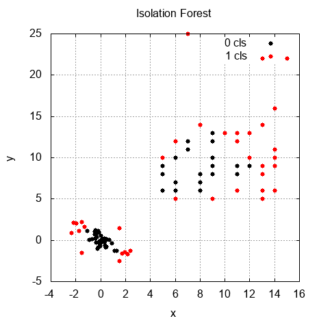
Finally, we called the AnomalyScore() method for each sample from the dataset in order to detect anomalies with thresholds and return their values. In the following graph, we can see the result of anomaly detection after using the Isolation Forest algorithm. The red points are the anomalies: