10
GRAPHICAL USER INTERFACES AND THE CANVAS

Before we dive into simulations, we need to understand the basics of graphical user interfaces (GUIs). This is a massive topic, and we’ll barely scratch the surface, but we’ll see enough for us to present our simulations to the user.

GUIs typically consist of a parent window (or windows) containing widgets the user can interact with, such as buttons or text fields. For our goal of drawing simulations, the widget we’re most interested in is the canvas. In a canvas we can draw geometric primitives, and we can redraw them many times per second, something that we’ll use to create the perception of motion.

In this chapter, we’ll cover how to lay out a GUI using Tkinter, a package shipped with Python’s Standard Library. Once we’ve got that down, we’ll implement a class that will make drawing our geometric primitives to the canvas convenient. This class will also include an affine transformation as part of its state. We’ll use this to affect how all primitives are drawn to the canvas, which will allow us to do things such as flip the drawing vertically so that the y-axis points up.

Tkinter

Tkinter is a package that ships with Python’s Standard Library. It’s used for building graphical user interfaces. It provides the visual components, in other words, the widgets, such as buttons, text fields, and windows. It also provides the canvas, which we’ll use to draw the frames of our simulations.

Tkinter is a feature-rich library; there are entire books written on it (see, for example, [7]). We’ll only cover what we need for our purposes, but if you enjoy creating GUIs, I recommend you spend some time looking through Tkinter’s documentation online; there’s a lot you can learn that will help you build fancy GUIs for your programs.

Our First GUI Program

Let’s create a new package in the graphic folder where we’ll place our simulation code. Right-click graphic, choose New ▸ Python Package, name it simulation, and click OK. The folder structure in your project should look like this:

        Mechanics
          |- apps
          |    |- circle_from_points
          |- geom2d
          |    |- tests
          |- graphic
          |    |- simulation
          |    |- svg
          |- utils

Let’s now create our first GUI program to get acquainted with Tkinter. In the newly created simulation folder, add a new Python file named hello_tkinter.py. Enter the code in Listing 10-1.

from tkinter import Tk

tk = Tk()
tk.title("Hello Tkinter")

tk.mainloop()

Listing 10-1: Hello Tkinter

To execute the code in the file, right-click it in the Project tree panel and choose Run ‘hello_tkinter’ from the menu that appears. When you execute the code, an empty window with the title “Hello Tkinter” opens, as shown in Figure 10-1.

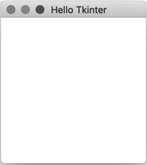
Figure 10-1: The empty Tkinter window

Let’s review the code we’ve just written. We start by importing the Tk class from tkinter. The tk variable holds an instance of Tk, which represents the main window in a Tkinter program. This window is also referred to as root in the documentation and examples online.

We then set the title of the window to Hello Tkinter and run the main loop. Notice that the main window won’t appear on the screen until the main loop starts. In a GUI program, the main loop is an infinite loop: it runs the entire time the program is being executed; as it runs, it collects user events in its windows and reacts to them.

Graphical user interfaces are different than the other programs we’ve been writing so far in that they’re event driven. This means that graphic components can be configured to run some code whenever they receive an event of the desired type. For example, we can tell a button to write a message when it receives a click event, that is, when it gets clicked. The code that reacts to an event is commonly known as an event handler.

Let’s add a text field where the user can write their name, and let’s add a button to greet them by name. Modify your hello_tkinter.py file to include the code in Listing 10-2. Pay attention to the new imports on top of the file.

  from tkinter import Tk, Label, Entry, Button, StringVar

  tk = Tk()
  tk.title("Hello Tkinter")

➊ Label(tk, text='Enter your name:').grid(row=0, column=0)
➋ name = StringVar()
➌ Entry(tk, width=20, textvariable=name).grid(row=1, column=0)
➍ Button(tk, text='Greet me').grid(row=1, column=1)

  tk.mainloop()

Listing 10-2: Hello Tkinter widgets

To add the label “Enter your name:” we’ve instantiated the Label class from tkinter ➊. We pass the constructor the reference to the program’s main window (tk) and a named argument with the text to display: text=’Enter your name:’. Before the label can appear in the window, we need to tell it where to place itself in the window.

On the created instance of Label, we call grid with the named arguments row and column. This method places the widget in an invisible grid in the window, in the given row and column indices. Cells in the grid adapt their size to fit their contents. As you can see in the code, we call this method on every widget to assign them a position in the window. Figure 10-2 shows our UI’s grid. There are other ways of placing components in windows, but we’ll use this one for now because it’s flexible enough for us to easily arrange components.

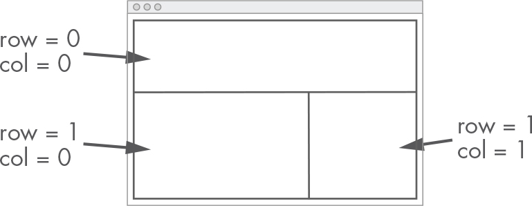
Figure 10-2: Tkinter grid

The input field in Tkinter is known as Entry ➌. To have access to the contents of the field (the text written to it), we must first create a StringVar, which we’ll call name ➋. This variable is passed to the Entry component using the textvariable argument. We can get the string written in the field by invoking get on the instance, as we’ll do shortly. Lastly, we create a button with the text “Greet me” ➍; this button does nothing if clicked (we’ll add that functionality shortly).

Run the file. You should now see a label, a text field, and a button, as in Figure 10-3.

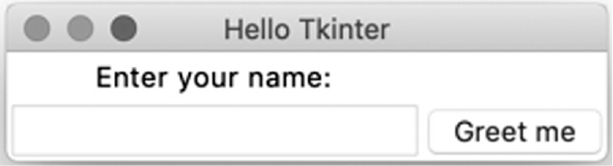
Figure 10-3: Some Tkinter widgets

Let’s finish our program by adding an event handler to the button’s click, which opens a new dialog with a greeting message. Modify your code so that it looks like Listing 10-3.

  from tkinter import Tk, Label, Entry, Button, StringVar, messagebox

  tk = Tk()
  tk.title("Hello Tkinter")

➊ def greet_user():
      messagebox.showinfo(
         'Greetings',
         f'Hello, {name.get()}'
      )


  Label(tk, text='Enter your name:').grid(row=0, column=0)
  name = StringVar()
  Entry(tk, width=20, textvariable=name).grid(row=1, column=0)
  Button(
     tk,
     text='Greet me',
   ➋ command=greet_user
  ).grid(row=1, column=1)

tk.mainloop()

Listing 10-3: Hello Tkinter that greets users

We’ve added a function named greet_user ➊. This function opens an information dialog with the title “Greetings” and a message saying hello to the name the user entered in the text field. Note that we import messagebox from tkinter to call the showinfo function. This function does the actual work of opening the dialog. To connect the button click event to our greet_user function, we need to pass it to Button’s constructor in a parameter named command ➋.

Run the file now. Don’t forget to close our application’s window and rerun the program every time you want your new code to be executed. Enter your name in the text field and click the button. The program should open a new dialog with a personalized greeting, something similar to Figure 10-4.

Figure 10-4: Our Tkinter greeter program

There’s much more Tkinter can do, but we won’t need that much for this book. We’re mostly interested in using its canvas component, which we’ll explore in the next section. If you want to learn more about Tkinter, you have lots of great resources online. You can also refer to [7], as mentioned earlier.

The Canvas

A canvas is a surface to paint on. In Tkinter’s digital world, it’s the same. The canvas component is represented by the Canvas class in tkinter.

Let’s create a new Tkinter application where we can experiment with drawing to the canvas. In the simulation folder, create a new file named hello_canvas.py and enter the code in Listing 10-4.

from tkinter import Tk, Canvas

tk = Tk()
tk.title("Hello Canvas")

canvas = Canvas(tk, width=600, height=600)
canvas.grid(row=0, column=0)

tk.mainloop()

Listing 10-4: Hello Canvas

The code creates a Tkinter application with its main window and a 600 by 600–pixel canvas. If you run the file, you should see an empty window with the title “Hello Canvas.” The canvas is there; it’s just that there’s nothing drawn yet.

Drawing Lines

Let’s start easy and draw a line on the canvas. Just between creating the canvas and starting the main loop, add the following line:

--snip--

canvas.create_line(0, 0, 300, 300)

tk.mainloop()

The arguments passed to create_line are, respectively, the x- and y-coordinates of the start point and the x- and y-coordinates of the end point.

Run the file again. There should be a line segment going from the upper-left corner, (0, 0), to the center of the screen, (300, 300). As you can guess, the origin of coordinates is in the upper-left corner of the screen with the y-axis pointing downward. Later when we’re animating simulations, we’ll use affine transformations to fix this.

By default, lines are drawn with a width of 1 pixel and painted in black, but we can change this. Try the following:

canvas.create_line(
    0, 0, 300, 300,
    width=3,
    fill='#aa3355'
)

The line is now thicker and has a reddish color. Your result should look like Figure 10-5.

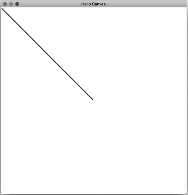
Figure 10-5: A line on a Tkinter canvas

Drawing Ovals

Let’s draw a circle in the middle of our application’s window using the same color as the previous line:

--snip--

canvas.create_oval(
    200, 200, 400, 400,
    width=3,
    outline='#aa3355'
)

tk.mainloop()

The arguments passed to create_oval are the x- and y-coordinates of the upper-left vertex of the rectangle that contains the oval, and the x- and y-coordinates of the lower-right vertex. These are followed by the named arguments used to determine the line’s width and color: width and outline.

If you run the file, you’ll see a circle in the center of the window. Let’s turn it into a proper oval by making it 100 pixels wider, maintaining its height of 400 pixels:

canvas.create_oval(
    200, 200, 500, 400,
    width=3,
    outline='#aa3355'
)

By changing the x-coordinate of the lower-right corner from 400 to 500, the circle turns into an oval. The application now has a canvas with both a line and an oval, as in Figure 10-6.

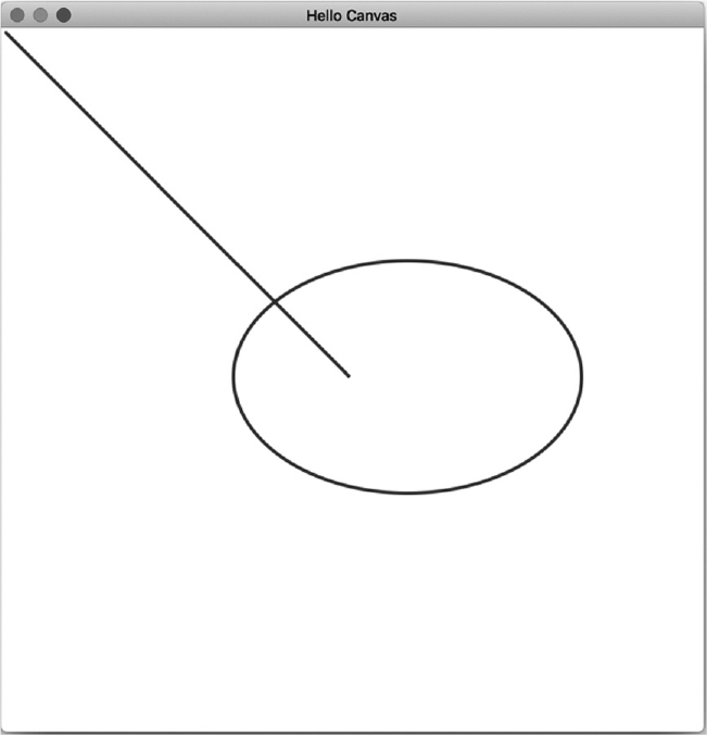
Figure 10-6: An oval added to our Tkinter canvas

If we wanted to add a fill color to the oval, we could do so using the named argument fill=’...’. Here’s an example:

canvas.create_oval(
    200, 200, 500, 400,
    width=3,
    outline='#aa3355',
    fill='#cc3355',
)

There’s one limitation, though: Tkinter doesn’t support transparency, which means all of our fills and strokes will be completely opaque. The color format #rrggbbaa where aa is the value for the alpha (transparency) is not supported in Tkinter.

Drawing Rectangles

Drawing rectangles is also pretty straightforward. Enter this code in the file:

--snip--

canvas.create_rectangle(
    40, 400, 500, 500,
    width=3,
    outline='#aa3355'
)

tk.mainloop()

The mandatory arguments to create_rectangle are the x- and y-coordinates of the upper-left corner of the rectangle and the x- and y-coordinates of the lower-right corner.

Run the file; the result should look like Figure 10-7.

Figure 10-7: A rectangle added to our Tkinter canvas

Nice! The resulting image is getting weirder, but isn’t it easy and fun to draw on the canvas?

Drawing Polygons

The last geometric primitive we need to know how to draw is a generic polygon. After the code you added to draw the rectangle, write the following:

--snip--

canvas.create_polygon(
    [40, 200, 300, 450, 600, 0],
    width=3,
    outline='#aa3355',
    fill=''
)

tk.mainloop()

The first parameter to create_polygon is a list of vertex coordinates. The rest are the named parameters that affect its style. Notice that we pass an empty string to the fill parameter; by default polygons get filled, but we want ours to be only an outline. Run the file to see the result. It should resemble Figure 10-8.

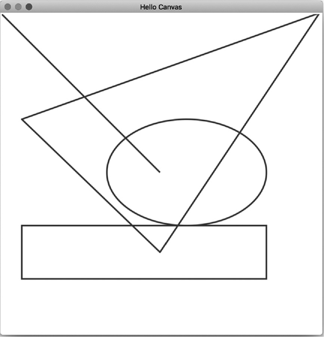
Figure 10-8: A polygon added to our Tkinter canvas

We created a triangle with vertices (40, 200), (300, 450), and (600, 0). Try adding a fill color and seeing what results.

Drawing Text

It isn’t a geometric primitive, but we may also need to draw some text to the canvas. Doing so is easy using the create_text method. Add the following to hello_canvas.py:

--snip--

canvas.create_text(
    300, 520,
    text='This is a weird drawing',
    fill='#aa3355',
    font='Helvetica 20 bold'
)

tk.mainloop()

The first two parameters are the x and y position for the center of the text. The named parameter text is where we set the actual text we want to draw; we can change its font using font. Run the file one last time to see the complete drawing, as shown in Figure 10-9.

If we can draw lines, circles, rectangles, generic polygons, and text, we can draw pretty much anything. We could also use arcs and splines, but we’ll manage to do our simulations using only these simple primitives.

Figure 10-9: Text added to our Tkinter canvas

Your final code should look like Listing 10-5.

from tkinter import Tk, Canvas

tk = Tk()
tk.title("Hello Canvas")

canvas = Canvas(tk, width=600, height=600)
canvas.grid(row=0, column=0)

canvas.create_line(
    0, 0, 300, 300,
    width=3,
    fill='#aa3355'
)
canvas.create_oval(
    200, 200, 500, 400,
    width=3,
    outline='#aa3355'
)
canvas.create_rectangle(
    40, 400, 500, 500,
    width=3,
    outline='#aa3355'
)
canvas.create_polygon(
    [40, 200, 300, 450, 600, 0],
    width=3,
    outline='#aa3355',
    fill=''
)
canvas.create_text(
    300, 520,
    text='This is a weird drawing',
    fill='#aa3355',
    font='Helvetica 20 bold'
)

tk.mainloop()

Listing 10-5: Final drawing code

Now that we know how to draw simple primitives to the canvas, let’s come up with a way of drawing our geom2d library’s geometric primitives directly to the canvas.

Drawing Our Geometric Primitives

Drawing a circle to the canvas was easy using its create_oval method. This method is, nevertheless, not convenient; to define the circle, you need to pass the coordinates of two vertices that define a rectangle where the circle or oval is inscribed. On the other hand, our class Circle is defined by its center point and radius, and it has some useful methods and can be transformed using instances of AffineTransform. It would be nice if we could directly draw our circles like so:

circle = Circle(Point(2, 5), 10)
canvas.draw_circle(circle)

We definitely want to work with our geometry primitives. Similar to how we created SVG representations of them in Chapter 8, we’ll need a way to draw them to the canvas.

Here’s the plan: we’ll create a wrapper for Tkinter’s Canvas widget. We’ll create a class that contains an instance of the canvas where we want to draw but whose methods allow us to pass our own geometric primitives. To leverage our powerful affine transformation implementation, we’ll associate a transformation to our drawing so that all primitives we pass will first be transformed.

The Canvas Wrapper Class

A wrapper class is simply a class that contains an instance of another class (what it’s wrapping) and is used to provide a similar functionality as the wrapped class, but with a different interface and some added functionality. It’s a simple yet powerful concept.

In this case, we’re wrapping a Tkinter canvas. Our canvas wrapper goal is to allow us to draw our geometric primitives with a simple and clean interface: we want methods that directly accept instances of our primitives. This wrapper will save us from the repetitive task of adapting the representation of the geometric classes to the inputs expected by the Tkinter canvas’s drawing methods. Not only that, but we’ll also apply an affine transformation to everything that we draw. Figure 10-10 depicts this process.

In the simulation package, create a new file named draw.py. Enter the code in Listing 10-6.

from tkinter import Canvas

from geom2d import AffineTransform


class CanvasDrawing:

    def __init__(self, canvas: Canvas, transform: AffineTransform):
        self.__canvas = canvas
        self.outline_color = '#aa3355'
        self.outline_width = 3
        self.fill_color = ''
        self.transform = transform

    def clear_drawing(self):
        self.__canvas.delete('all')

Listing 10-6: Canvas wrapper class

The class CanvasDrawing is defined as a wrapper to the Tkinter canvas. An instance of the canvas is passed to the initializer and stored in a private variable, __canvas. Making __canvas private means we don’t want anyone using CanvasDrawing to access it directly. It now belongs to the wrapper class instance, and it should only be used with its methods.

An instance of AffineTransform is also passed to the initializer. We’ll apply this affine transformation to all geometric primitives before we draw them to Tkinter’s canvas. The transformation is stored in a public variable: transform. This means we’re allowing users of CanvasDrawing instances to directly manipulate and edit this property, which is part of the state of the instance. We do this so that it’s simple to alter the affine transformation applied to the drawing, by reassigning the transform property to a different transformation.

The state of an instance defines its behavior: if the state changes, the instance’s behavior changes as well. In this case, it’s clear that if the property transform is reassigned a different affine transformation, all subsequent drawing commands will produce results in accordance with it.

Figure 10-10 is a diagram representing the behavior of our canvas wrapper class. It’ll receive draw requests for different geometric primitives, apply the affine transformation to them, and then call the Tkinter’s canvas methods to draw into it.

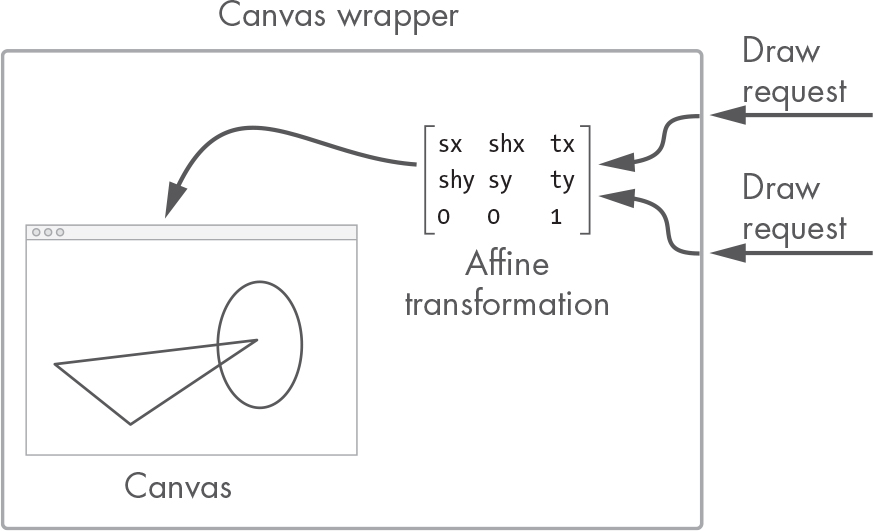
Figure 10-10: The canvas wrapper class

There are other state variables defined in the initializer: outline_color, which defines the color used for the outline of geometries, outline_width for the width of the outlines, and fill_color for the color used to fill the geometries. These are given default values in the initializer (those used in our example in the previous section) but are also public and accessible for users of the instance to change them. Like before, it should be clear that these properties are part of the state of the instance: if we edit outline_color, for example, all subsequent drawings will use that color for the outlines.

We’ve defined only one method in the class: clear_drawing. This method will clean the canvas for us before drawing each of the frames. Let’s now focus on the drawing commands.

Drawing Segments

Let’s start with the simplest primitive to draw: the segment. In the Canvas Drawing class, enter the method in Listing 10-7. For this code you first need to update the imports from geom2d to include the Segment class.

from tkinter import Canvas

from geom2d import Segment, AffineTransform


class CanvasDrawing:
   --snip--

   def draw_segment(self, segment: Segment):
       segment_t = self.transform.apply_to_segment(segment)
       self.__canvas.create_line(
           segment_t.start.x,
           segment_t.start.y,
           segment_t.end.x,
           segment_t.end.y,
           fill=self.outline_color,
           width=self.outline_width
       )

Listing 10-7: Drawing a segment

The draw_segment method does two things: first it transforms the given segment using the current affine transformation and stores the result in segment_t. Then it calls the create_line method from the canvas instance. For the outline color and width, we use the state variables of the instance.

Let’s move on to polygons, circles, and rectangles.

Drawing Polygons

If you recall from “Transform Segments and Polygons” on page 179, once an affine transformation is applied to a circle or rectangle, the result is a generic polygon. This means that all three polygons will be drawn using the create_polygon method from the canvas.

Let’s create a private method that draws a polygon to the canvas, forgetting about the affine transformation; that part will be handled by each of the public drawing methods.

In your CanvasDrawing class, enter the private method in Listing 10-8.

from functools import reduce
from tkinter import Canvas

from geom2d import Polygon, Segment, AffineTransform


class CanvasDrawing:
    --snip--

    def __draw_polygon(self, polygon: Polygon):
        vertices = reduce(
            list.__add__,
            [[v.x, v.y] for v in polygon.vertices]
        )

        self.__canvas.create_polygon(
            vertices,
            fill=self.fill_color,
            outline=self.outline_color,
            width=self.outline_width
        )

Listing 10-8: Drawing a polygon to the canvas

For this code you need to add the following import,

from functools import reduce

and update the imports from geom2d:

from geom2d import Polygon, Segment, AffineTransform

The __draw_polygon method first prepares the vertex coordinates of the polygon to meet the expectations of the canvas widget’s create_polygon method. This is done by reducing a list of lists of vertex coordinates with Python’s list __add__ method, which, if you recall, is the method that overloads the + operator.

Let’s break this down. First, the polygon’s vertices are mapped using a list comprehension:

[[v.x, v.y] for v in polygon.vertices]

This creates a list with the x- and y-coordinates from each vertex. If the vertices of the polygon were (0, 10), (10, 0), and (10, 10), the list comprehension shown earlier would result in the following list:

[[0, 10], [10, 0], [10, 10]]

This list then needs to be flattened: all values in the inner lists (the numeric coordinates) have to be concatenated into a single list. The result of flattening the previous list would be as follows:

[0, 10, 10, 0, 10, 10]

This is the list of vertex coordinates the method create_polygon expects. This final flattening step is achieved by the reduce function; we pass it the list .__add__ operator, and it produces a new list that results from concatenating both list operands. To see that in action, you can test the following in Python’s shell:

>>> [1, 2] + [3, 4]
[1, 2, 3, 4]

Once the list of vertex coordinates is ready, drawing it to the canvas is straightforward: we simply pass the list to the canvas’s create_polygon method. Now that the hardest part is done, drawing our polygons should be easier. Enter the code in Listing 10-9 to your class.

from functools import reduce
from tkinter import Canvas

from geom2d import Circle, Polygon, Segment, Rect, AffineTransform


class CanvasDrawing:
    --snip--

   def draw_circle(self, circle: Circle, divisions=30):
       self.__draw_polygon(
           self.transform.apply_to_circle(circle, divisions)
       )

   def draw_rectangle(self, rect: Rect):
       self.__draw_polygon(
           self.transform.apply_to_rect(rect)
       )

   def draw_polygon(self, polygon: Polygon):
       self.__draw_polygon(
           self.transform.apply_to_polygon(polygon)
       )

Listing 10-9: Drawing circles, rectangles, and generic polygons

Don’t forget to add the missing imports from geom2d:

from geom2d import Circle, Polygon, Segment, Rect, AffineTransform

In all three methods, the process is the same: call the private method __draw_polygon and pass it the result of applying the current affine transformation to the geometry. Don’t forget that in the case of a circle, we need to pass the number of divisions we’ll use to approximate it to the transform method.

Drawing Arrows

Let’s now draw arrows following the same approach we used in Chapter 8 for SVG images.

The arrow’s head will be drawn on the end point E of a segment and will be made of two segments at an angle meeting at such an end point. To allow some flexibility, we’ll use two dimensions to define the arrow’s geometry: a length and a height (see Figure 10-11).

As you can see in Figure 10-11 (repeated from Chapter 8), to draw the arrow’s head, we need to figure out points C₁ and C₂. With those two points, we can easily draw the segments between C₁ and E and between C₂ and E.

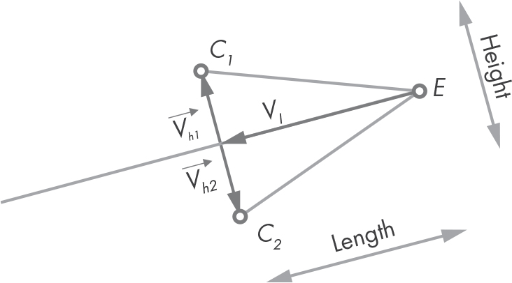
Figure 10-11: Key points in an arrow

To find out where those points lie in the plane, we’ll be computing three vectors: , which has the same length as the arrow’s head and is going in the opposite direction of the segment’s direction vector, and and , which are perpendicular to the segment and both have a length equal to half the arrow’s head height. Figure 10-11 shows these vectors. The point C₁ can be computed by creating a displaced version of E (the segment’s end point),

and similarly, C₂:

Let’s write the method. In the CanvasDrawing class, enter the code in Listing 10-10.

class CanvasDrawing:
    --snip--

    def draw_arrow(
            self,
            segment: Segment,
            length: float,
            height: float
    ):
        director = segment.direction_vector
        v_l = director.opposite().with_length(length)
        v_h1 = director.perpendicular().with_length(height / 2.0)
        v_h2 = v_h1.opposite()

        self.draw_segment(segment)
        self.draw_segment(
            Segment(
                segment.end,
             ➊ segment.end.displaced(v_l + v_h1)
            )
        )
        self.draw_segment(
            Segment(
                segment.end,
             ➋ segment.end.displaced(v_l + v_h2)
            )
        )

Listing 10-10: Drawing an arrow

We start by computing the three vectors we need to figure out points C₁ and C₂ using the previous equations. As you can see, this is pretty straightforward thanks to the methods we implemented in our Vector class. For example, to obtain , we use the opposite vector of the segment’s direction vector and scale it to have the desired length. We use similar operations to calculate the remaining elements of our equations.

Then we three segments: the base line, which is the segment passed as the argument; the segment going from E to C₁ ➊ ; and the one going from E to C₂ ➋.

For reference, your drawing.py file should look like Listing 10-11.

from functools import reduce
from tkinter import Canvas

from geom2d import Circle, Polygon, Segment, Rect, AffineTransform


class CanvasDrawing:

    def __init__(self, canvas: Canvas, transform: AffineTransform):
        self.__canvas = canvas
        self.outline_color = '#aa3355'
        self.outline_width = 3
        self.fill_color = ''
        self.transform = transform

    def clear_drawing(self):
        self.__canvas.delete('all')

    def draw_segment(self, segment: Segment):
        segment_t = self.transform.apply_to_segment(segment)
        self.__canvas.create_line(
            segment_t.start.x,
            segment_t.start.y,
            segment_t.end.x,
            segment_t.end.y,
            outline=self.outline_color,
            width=self.outline_width
        )

    def draw_circle(self, circle: Circle, divisions=30):
        self.__draw_polygon(
            self.transform.apply_to_circle(circle, divisions)
        )

    def draw_rectangle(self, rect: Rect):
        self.__draw_polygon(
            self.transform.apply_to_rect(rect)
        )

    def draw_polygon(self, polygon: Polygon):
        self.__draw_polygon(
            self.transform.apply_to_polygon(polygon)
        )

    def __draw_polygon(self, polygon: Polygon):
        vertices = reduce(
            list.__add__,
            [[v.x, v.y] for v in polygon.vertices]
        )

        self.__canvas.create_polygon(
            vertices,
            fill=self.fill_color,
            outline=self.outline_color,
            width=self.outline_width
        )

    def draw_arrow(
            self,
            segment: Segment,
            length: float,
            height: float
    ):
        director = segment.direction_vector
        v_l = director.opposite().with_length(length)
        v_h1 = director.perpendicular().with_length(height / 2.0)
        v_h2 = v_h1.opposite()

        self.draw_segment(segment)
        self.draw_segment(
            Segment(
                segment.end,
                segment.end.displaced(v_l + v_h1)
            )
        )
        self.draw_segment(
            Segment(
                segment.end,
                segment.end.displaced(v_l + v_h2)
            )
        )

Listing 10-11: CanvasDrawing class result

We now have a convenient way of drawing our geometric primitives, but they’re not moving at all, and we need motion to produce simulations. What’s the missing ingredient to bring those geometries to life? That’s the topic of the next chapter. Matters are getting more and more exciting!

Summary

In this chapter, we covered the basics of creating graphical user interfaces using Python’s Tkinter package. We saw how to lay widgets on the main window using the grid system. We also learned how to make a button respond to being clicked and how to read the contents of a text field. Most importantly, we learned about the Canvas class and its methods that we can use to draw simple primitives to it.

We finished the chapter by creating a class of our own that wraps Tkinter’s canvas and allows us to draw our geometric primitives directly. The class also includes an affine transformation that applies to the primitives before being drawn. The class has properties that define the stroke width and color as well as the fill color. These are the width and colors applied to the primitives we draw with it. Now it’s time to put those static geometries into motion.