
INTRODUCTION

Knowing how to write code empowers you to solve complex problems. By harnessing the capabilities of modern CPUs, which can accomplish billions of operations per second, we can quickly and correctly work out the solutions to difficult problems.
This is a book about solving engineering problems with Python. We’ll learn how to code geometric primitives that will serve as the basis of more complex operations, how to read and write from files, how to create vector images and animated sequences to present the results, and how to solve large systems of linear equations. Finally, we’ll put all this knowledge together to build an application that solves truss structure problems.
Who This Book Is For
This book is targeted at engineering students, graduated engineers, or just about any person with a technical background who wants to learn how to write applications to solve engineering problems.
A background in math and mechanics is a must. We’ll be using concepts from linear algebra, 2D geometry, and physics. We’ll also use some mechanics of materials and numerical methods, which are subjects common to many engineering degrees. We won’t go too far into these topics to allow a larger number of readers to find the material of the book useful. The techniques learned in this book can later be used to solve problems that involve more complex concepts.
To follow along, you’ll need to have some coding skills and basic Python knowledge. This is not an introductory book to programming; there are lots of other good books covering that. I can recommend Python Crash Course by Eric Matthes (No Starch Press, 2019) if you’re looking for such a book. There’s also a lot of great material online, from which I’d pick https://realpython.com as my favorite. The official Python website is also full of good tutorials and documents: https://www.python.org/about/gettingstarted/.
We’re going to write a lot of code, so I strongly recommend you have a computer with you as you read and that you enter and test all the code in this book.
What You’ll Learn
In this book, we’ll explore techniques to write robust applications that correctly, and quickly, solve engineering problems. To ensure correctness, we’ll be testing our code using automated tests. Every application you build should be properly tested using automated testing, as we’ll discuss throughout the book.
Engineering applications usually require some amount of data to be fed in, so we’ll also learn how to read the input of our programs from a file, parsing it using regular expressions.
Engineering applications typically need to solve a large system of equations, so we’ll cover how to write numerical methods that can do these complex computations. We’ll focus on linear systems, but the same techniques can easily be applied to write numerical algorithms for nonlinear equations.
Lastly, engineering applications need to produce a result. We’ll learn how to write text to files that we can later inspect. We’ll cover how to produce beautiful vector diagrams and animated sequences to present the results of our programs. As they say, a diagram is worth a thousand words: looking at a well-drawn diagram that describes the result with the most relevant solution values makes programs much more valuable.
To illustrate all these concepts, we’ll conclude the book by building an application that solves two-dimensional truss structures. This application will have everything you need to build engineering applications. The knowledge acquired building this application can easily be translated to writing other kinds of engineering applications.
About This Book
In this section, we’ll explain three things: the meaning behind the title of this book, the choice of Python, and the table of contents.
What Is the “Hardcore” About?
The word Hardcore in the title of this book refers to the fact that we’ll write all the code ourselves, relying only on the Python standard libraries (libraries that ship with Python); we won’t use any third-party library to solve equations or draw vector images.
You may be wondering why. If there’s code already written by someone that does all this for us, why not simply use it? Aren’t we re-inventing the wheel?
This is a book about learning, and to learn you need to do things yourself. You’ll never understand the wheel unless you re-invent it. Once your software skills are solid and you’ve written thousands of lines of code and worked on a lot of projects, you’ll be in a good position to decide which external libraries fit your needs and how to leverage them. But if you use those libraries from the beginning, you’ll get used to using them and take the solutions for granted. It’s important to always ask yourself, how does this library’s code work to solve my problem?
Like anything else, coding takes practice. If you want to become good at coding, you need to write a lot of code; there are no shortcuts. If you’re getting paid to write software or want to take an idea to market as fast as possible, then use existing libraries. But if you’re learning and want to become proficient in the art of writing code, don’t use libraries. Write the code yourself.
Why Python?
Python is one of the most beloved programming languages. According to Stack Overflow’s 2020 developer survey (https://insights.stackoverflow.com/survey/2020), Python is today’s third most loved language, with 66.7 percent of its users willing to continue using it in the future, just behind TypeScript and Rust (see Figure 1).

Figure 1: 2020 most loved languages (source: Stack Overflow survey)
This same survey puts Python first when it comes to “desired” languages: 30 percent of the surveyed developers who are not currently using Python expressed interest in learning it (see Figure 2).
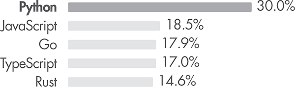
Figure 2: 2020 most wanted languages (source: Stack Overflow survey)
These results are not surprising; Python is an extremely versatile and productive language. Writing code in Python is a delight, and its Standard Library is well equipped: for just about anything you want to do, Python has something ready to help.
We’ll use Python in this book not only because of its popularity but also because it’s easy to use and versatile. One nice thing about Python is that, if you are reading this book but have no prior knowledge of the language, it won’t take you long to get started. It’s a relatively easy language to learn and the internet is filled with tutorials and courses to help you.
What Python is typically not seen as is a fast language, and indeed, Python’s execution times are not one of its strengths. Figure 3 below shows a comparison of the execution times in seconds of the same three programs written both in Python and in Go (a very fast language developed by Google). In every case, Python takes much longer than Go to execute.
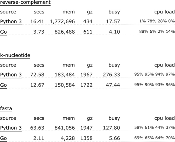
Figure 3: Python benchmark (source: https://benchmarksgame-team.pages.debian.net/benchmarksgame/fastest/python3-go.html)
So, don’t we care about speed? We do, but for the purposes of this book, we care more about development time and the development experience. Python has lots of constructs that make coding delightful; for example, things like filtering or mapping a collection can be done out of the box using Python’s list comprehensions, whereas in Go, you need to do those operations using good old for loops. For almost every program we’ll write, execution time will never be a concern, as we’ll get more than acceptable results. The skills you learn in this book will transfer to other, faster languages if you encounter speed issues in your applications.
But before we start learning anything, let’s have a quick overview of the topics you’ll find in this book.
Contents at a Glance
We’ll cover a lot of ground in this book. Each chapter builds on top of the previous ones, so you’ll want to make sure to read the book in order and work on the code each chapter presents.
The book includes the following chapters:
Chapter 1: A Short Python Primer Introduces some intermediate Python topics that we’ll use throughout the book. We’ll cover how to split our code into modules and packages, how to use Python’s collections, and how to run Python scripts and import modules.
Chapter 2: Two Python Paradigms Covers functional and object-oriented programming paradigms and explores techniques to write code in those styles.
Chapter 3: The Command Line Instructs you on how to use the command line to run programs and other simple tasks such as creating files.
Chapter 4: Points and Vectors Covers the most basic, but crucial, geometric primitives: points and vectors. The rest of the book relies on the implementation of these two primitives, so we’ll also learn about automated testing to make sure our implementations are bug-free.
Chapter 5: Lines and Segments Adds the line and segment geometric primitives to our geometry toolbox. We’ll take a look at how to check whether two segments or two lines intersect and how to calculate the intersection points.
Chapter 6: Polygons Adds rectangles, circles, and generic polygons to our geometry toolbox.
Chapter 7: Affine Transformations Covers affine transformations, an interesting algebraic construct we’ll use to produce beautiful images and animations.
Part III: Graphics and Simulations
Chapter 8: Drawing Vector Images Introduces the Scalable Vector Graphics (SVG) image format. We’ll write our own library to produce these images using our geometric primitives.
Chapter 9: Building a Circle from Three Points Takes all the knowledge from the previous chapters to build our first application, one that finds the circle that goes through three given points and draws the result to a vector image.
Chapter 10: Graphical User Interfaces and the Canvas Covers the basics of the Tkinter package, which is used to build user interfaces in Python. We’ll spend most of the time learning how to use the Canvas widget, which is used to draw images to the screen.
Chapter 11: Animations, Simulations, and the Time Loop Guides you through the process of creating an animation by drawing inside Tkinter’s Canvas. We’ll explore the concept of the time loop used by engineering simulations and video game engines to render scenes to the screen.
Chapter 12: Animating Affine Transformations Creates an application that animates the effect of applying an affine transformation to some geometric primitives.
Chapter 13: Matrices and Vectors Introduces the vector and matrix constructs and covers how to code these primitives, which will be extremely useful when we’re working with systems of equations.
Chapter 14: Linear Equations Shows how numerical methods can be implemented to solve large systems of linear equations. We’ll implement the Cholesky factorization method together; this algorithm will solve the systems of equations that will appear in the next and last part of the book.
Chapter 15: Structural Models Reviews the basic mechanics of materials concepts we’ll use in this part of the book. We’ll also write the classes to represent a truss structure. Using this truss structure model we’ll build a complete structural analysis application.
Chapter 16: Structure Resolution Using the model built in the previous chapter, we’ll cover all the computations required to find the structure’s displacements, deformations, and stresses.
Chapter 17: Reading Input from a File Covers the implementation of file reading and parsing so that our truss analysis application can rely on data that’s stored as plaintext.
Chapter 18: Producing an SVG Image and Text File Discusses the generation of SVG image diagrams based on the structure solution. Here we’ll use our own SVG package to draw the diagrams, which will contain all the relevant details such as the geometry of the deformed structure and the stress label next to each bar.
Chapter 19: Assembling Our Application Explains how to put together the pieces built in the previous chapters to build the complete truss resolution application.
Setting Up Your Environment
In this book, we’ll use Python 3 and provide instructions to work with PyCharm, a development environment program that’ll let us work effectively. The code has been tested using Python versions 3.6 through 3.9, but it’ll most likely continue to work equally well with future versions of the language. Let’s download the code that accompanies the book, install the latest Python 3 interpreter, and set up PyCharm.
Downloading the Book’s Code
All the code for this book is available on GitHub at https://github.com/angelsolaorbaiceta/Mechanics. Again, while I strongly recommend that you write all the code yourself, it’s a good idea to have it with you for reference.
If you are familiar with Git and GitHub, you may want to clone the repository. Also, I suggest fetching and pulling from the repository from time to time, as I may add new features or fix bugs in the project.
If you are not familiar with the Git version control system or GitHub, your best option is to download a copy of the code. You can do this by clicking the Clone button and choosing the Download ZIP option (see Figure 4).
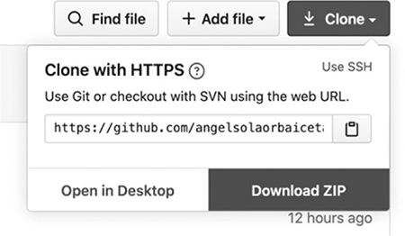
Figure 4: Downloading the code from GitHub
Unzip the project and place it inside the directory of your choice. As you’ll see, I documented every package and subpackage in the project using README files (README.md). These files are usually found in software projects; they explain and document the features of a project and also include instructions on how to compile or run the code. A README file is the first thing you want to read when you open a software project, as they describe how to configure the project and get the code running.
NOTE
README files are written using the Markdown format. If you want to know more about this format, you can read about it here: https://www.markdownguide.org/.
The Mechanics project on GitHub contains more code than we cover in this book. We didn’t want to make this book too long, so we couldn’t cover everything included in the project.
For example, in Chapter 14, “Linear Equations,” we talk about numerical methods to solve systems of linear equations and explain the Cholesky factorization in detail. There are some other numerical methods in the project, such as the conjugate gradient, which we don’t have time to cover in the book; the code is there for you to analyze and use. There are also many automated tests that we skip in the book for brevity reasons; use those tests as a reference when you write your own.
It’s time to install Python.
Installing Python
You can download Python for macOS, Linux, and Windows from https://www.python.org/downloads/. For Windows and macOS you’ll need to download the installer and run it.
Linux typically comes with Python preinstalled. You can check which version is installed on your computer using the following command in the shell:
$ python3 -V
Python 3.8.2
To install a version of Python on a Linux computer, you use the os package manager. For Ubuntu users using the apt package manager, this would be
$ sudo apt install python3.8
For Fedora users, using the dnf package manager, this would be
$ sudo dnf install python38
If you are using a different Linux distribution, a quick Google search should get you the instructions to install Python using your package manager.
It’s important that you download a version of Python 3, such as 3.9, which is the current version at the time of writing. Any version above 3.6 (included) will work.
NOTE
Python versions 2 and 3 are not compatible; code written targeting Python 3 will very likely not work with Python’s version 2 interpreter. The language evolved in a non-backwards-compatible way, and some features in version 3 are not available in version 2.
Installing and Configuring PyCharm
As we develop our code, we’ll want to use an integrated development environment (or IDE for short), a program equipped with features that help us write code more effectively. An IDE typically offers autocompletion features to let you know what options you have available as you type, as well as build, debug, and test tools. Taking some time to learn the main features of your IDE of choice is worth the effort: it’ll make you much more productive during the development phase.
For this book we’ll be using PyCharm, a powerful IDE created by JetBrains, a company that makes not only some of the best IDEs on the market but also its own programming language: Kotlin. If you already have some Python experience and prefer to use another IDE, such as Visual Studio Code, you’re welcome to do so, but you’ll need to figure out some things on your own using your IDE’s documentation. If you don’t have a lot of previous experience with any IDE, I recommend you stick to using PyCharm so you can follow along with the book.
To download PyCharm, head to https://www.jetbrains.com/pycharm/ and click the Download button (see Figure 5).

Figure 5: Downloading PyCharm IDE
PyCharm is available for Linux, macOS, and Windows. It has two different versions: Professional and Community. You can download the Community version for free. Follow the installer steps to install PyCharm on your machine.
Opening the Mechanics Project
Let’s use PyCharm to set up the Mechanics project you downloaded earlier so you can play with it and have its code for reference.
Open PyCharm and click the Open option on the welcome screen. Locate the Mechanics project folder you downloaded or cloned from GitHub and select it. PyCharm should open the project and configure a Python interpreter for it, using the version of Python installed in your computer.
Every project inside PyCharm requires that a Python interpreter be set. Since you could have several different versions of Python installed on your machine and because you may have chosen custom install locations, you need to tell PyCharm which of those versions of Python you want to use to interpret your project’s code and where to find Python’s interpreter in your system. For Windows and Linux users, go the menu and choose File ▸ Settings. For macOS users, choose PyCharm ▸ Preferences. In the Settings/Preferences window, click the Project: Mechanics section in the left column to expand it and choose Python Interpreter (see Figure 6).
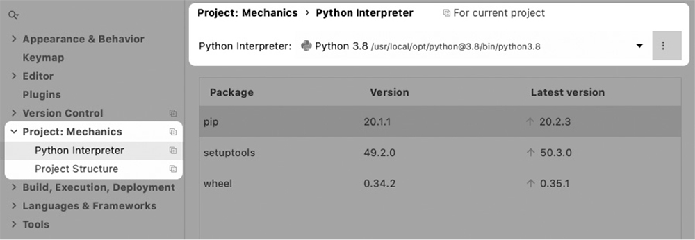
Figure 6: Setting up the project’s Python interpreter
On the right side of the window, click the down arrow beside the Python Interpreter field, and from the drop-down, choose the version of the Python binary you installed on your computer. If you followed the previous instructions, Python should have been installed to a default directory where PyCharm can find it, so the interpreter should appear in the list. If you’ve installed Python somewhere else, you’ll need to tell PyCharm the directory where you did so.
NOTE
If you have any trouble setting the project’s interpreter, check PyCharm’s official documentation: https://www.jetbrains.com/help/pycharm/configuring-python-interpreter.html. This link contains a detailed explanation of the process.
Now that you’ve opened the Mechanics project, it should already be set up. Open the README.md file inside PyCharm by double-clicking it. By default, when you open a Markdown file in PyCharm, it’ll show you a split view: to your left is the Markdown raw file and to your right is the rendered version of the file. See Figure 7.
This README.md file explains the basic structure of the project. Feel free to navigate through the links in the preview; give yourself some time to read through the README files inside each of the packages. This will give you a good sense of the amount of work we’ll do together throughout the book.

Figure 7: README.md file with PyCharm’s split view
Creating Your Own Mechanics Project
Now that you have the Mechanics project you downloaded set up for reference, let’s create a new empty project where you can write your code. Close the project if you have it open (select File ▸ Close Project). You should see the welcome page, as in Figure 8.
Figure 8: PyCharm welcome screen
From the welcome page choose Create New Project. You’ll be asked to name your project: use Mechanics. Then, for the interpreter, instead of the default, which is New environment using, select the Existing interpreter option (see Figure 9). Locate the version of Python you downloaded earlier in the introduction and click CREATE.
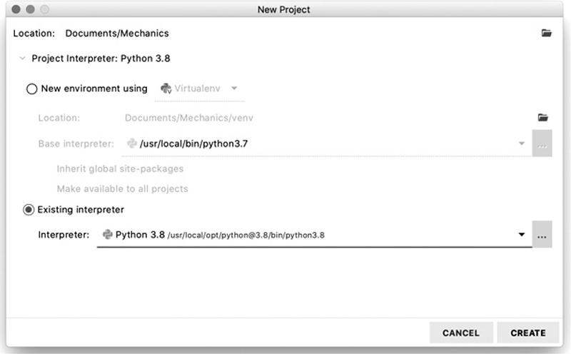
Figure 9: PyCharm, creating a new project
You should have a new empty project created and ready for you to write code. Let’s take a quick look at PyCharm’s main features.
PyCharm Introduction
This section is by no means a thorough guide to using PyCharm. To get a more complete overview of the IDE, you should read the documentation at https://www.jetbrains.com/help/pycharm. The official documentation is complete and up-to-date with the latest features.
PyCharm is a powerful IDE, and its Community (free) version even comes packed with lots of functionality; it makes working with Python a delightful experience. Its user interface (UI) can be divided into four main sections (see Figure 10).
Navigation bar On the top of the window is the navigation bar. To its left is the breadcrumb navigation of the currently open file. To its right are buttons to run and debug the program, as well as the drop-down list that shows the current run configuration (we’ll cover run configurations later in the book).
Project Tool window This is the directory structure of your project, including all its packages and files.
Editor This is where you’ll write your code.
Terminal PyCharm comes with two terminals: your system’s terminal and Python’s terminal. We’ll use both of them throughout the book. We’ll cover these in Chapter 3.
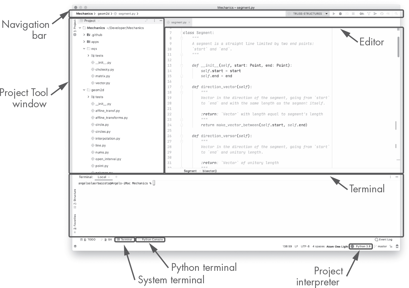
Figure 10: PyCharm UI
PyCharm also includes the project’s Python interpreter in the lower-right corner of the UI. You can change the interpreter’s version from here, choosing from a list of versions installed on your system.
Creating Packages and Files
We can create new Python packages (we’ll cover packages in Chapter 1) in your project using the Project Tool window. To create a new package, go to the Project Tool window and right-click the folder or package where you want to create the new package; from the menu that appears, select New ▸ Python Package. Similarly, select New ▸ Python File to create Python files. You can see these options in Figure 11.
You can also create regular directories with New ▸ Directory and all types of files using New ▸ File, which will let you choose the file’s extension yourself. The difference between a regular directory and a Python package is that the latter includes a file named __init__.py that instructs Python’s interpreter to understand the directory as a package with Python code. You’ll learn more about this in Chapter 1.
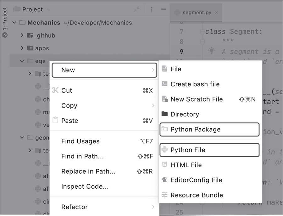
Figure 11: PyCharm new package or file
Creating Run Configurations
A run configuration is just a way of telling PyCharm how we want our project (or a part of it) to run. We can save this configuration to use as many times as we need. With a run configuration in place, we can execute our application by simply pressing a button, as opposed to having to write a command in the shell, which potentially entails copy-pasting parameters, inputting filenames, and the like.
Among other things, a run configuration can include information about the entry point for our application, what files to redirect to the standard input, what environment variables have to be set, and what parameters to pass to the program. Run configurations are a convenience that will save us time when developing; they also allow us to easily debug Python code, as we’ll see in the next section. You can find the official documentation for run configurations here: https://www.jetbrains.com/help/pycharm/run-debug-configuration.html.
Let’s create a run configuration ourselves to get some hands-on experience. To do this, let’s first create a new empty project.
Creating a Test Project
To create a new project from the menu, choose File ▸ New Project. In the Create Project dialog, enter RunConfig for the project’s name, select the Existing interpreter option, and then click CREATE.
In this new empty project, add a Python file by right-clicking the RunConfig empty directory in the Project Tool window and then selecting New ▸ Python File. Name it fibonacci. Open the file and enter this code:
def fibonacci(n):
    if n < 3:
        return 1

    return fibonacci(n - 1) + fibonacci(n - 2)


fib_30 = fibonacci(30)
print(f'the 30th Fibonacci number is {fib_30}')
We’ve written a function to compute the nth Fibonacci number using a recursive algorithm, which we then use to compute and print the 30th number. Let’s create a new run configuration to execute this script.
Creating a New Run Configuration
To create a new run configuration, from the menu select Run ▸ Edit Configurations; the dialog in Figure 12 should appear.
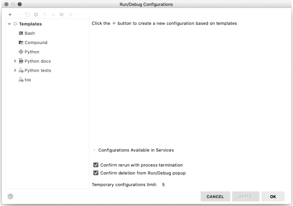
Figure 12: The Run/Debug Configurations dialog
As you can see, there are a few templates we can use to create a new run configuration. Each template defines parameters to help us readily create the right kind of configuration. We’re only going to use the Python template in this book. This template defines a run configuration to run and debug Python files.
In the dialog, click the + button in the top-left corner and select Python from the list of available templates (see Figure 13).
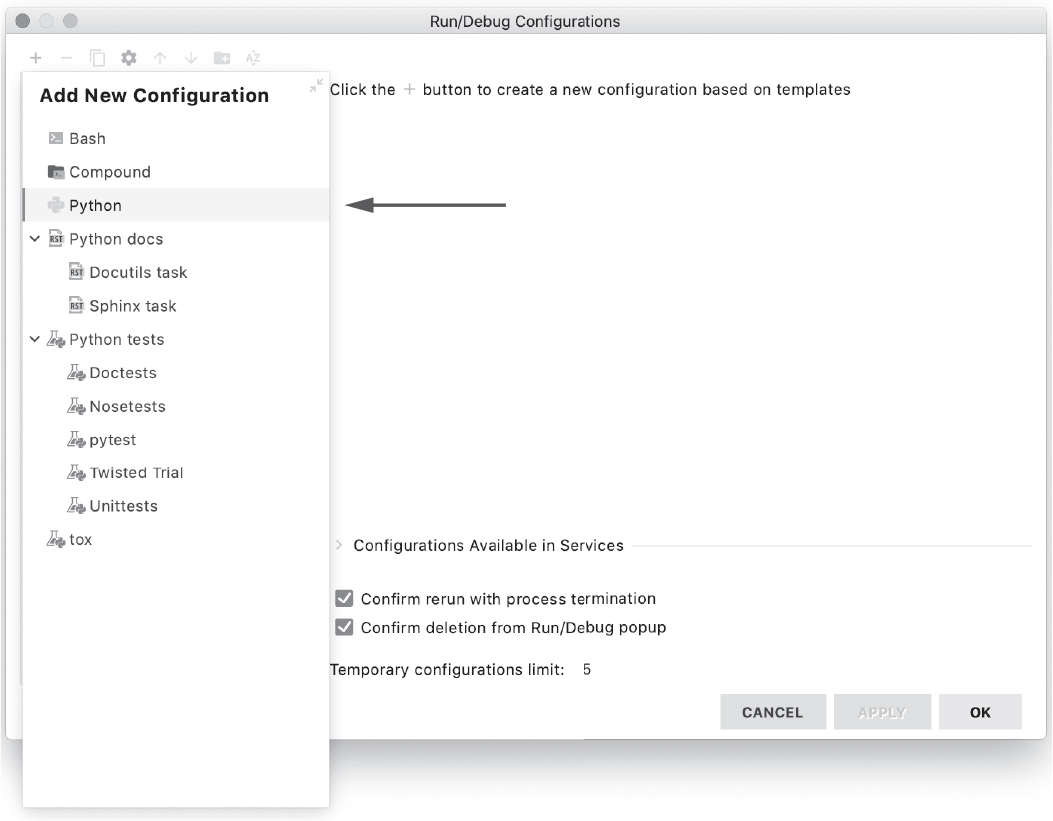
Figure 13: Creating a new Python run configuration
Once you’ve chosen the configuration template, the right side of the dialog displays the parameters we’ll need to provide for this configuration to run our code. We only need to fill two of these parameters: the configuration’s name and the script path.
Locate the Name field at the top of the dialog and enter fibonacci. Then locate the Script path field under the Configuration section, and click the folder icon to its right. Upon clicking this icon, a file dialog should open inside the project’s root folder, exactly where we’ve added our fibonacci.py file. Choose this file as the script path. Your new configuration dialog should look similar to Figure 14. Click OK.
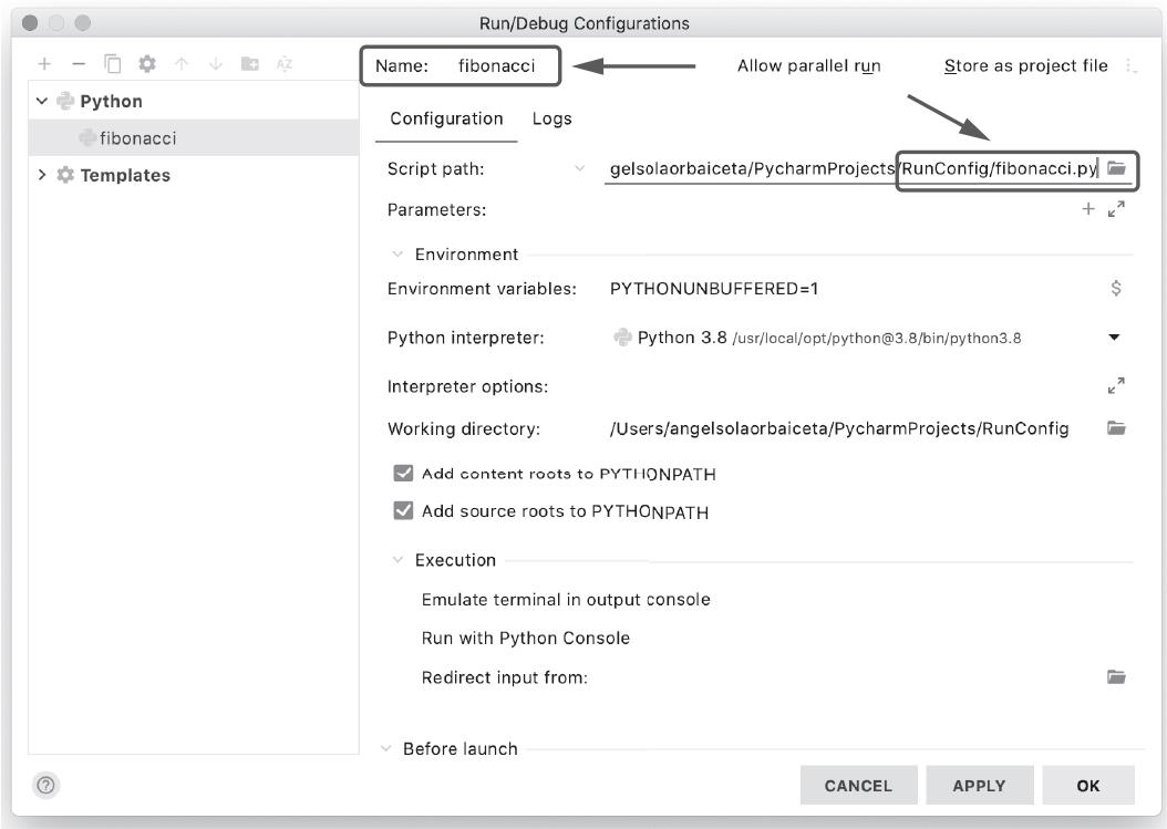
Figure 14: The run configuration parameters
You’ve successfully created a run configuration. Let’s use it.
Using the Run Configuration
In the navigation bar, toward the right, locate the run configuration selector. Figure 15 shows this selector.
Figure 15: The run configuration selector
In the drop-down list, select the run configuration you just created and click the green play button to execute it. You should see the following message in the shell of the IDE:
the 30th Fibonacci number is 832040

Process finished with exit code 0
You can also launch a run configuration from the menu by selecting Run ▸ Run ‘fibonacci’.
We’ve successfully used a run configuration to launch our fibonacci.py script. Let’s now use it to learn about debugging Python code.
Debugging Python Code
When our programs are misbehaving and we don’t know why, we can debug them. To debug a program, we can execute it line by line, one step at a time, and inspect the values of the variables.
Let’s modify our fibonacci function a little bit before we debug the script. Imagine that the users of this function are complaining about it being too slow for large numbers. For example, they state they have to wait several minutes for the function to compute the 50th Fibonacci number:
# this will fry your CPU... be prepared to wait
>>> fibonacci(50)
After careful analysis, we realize that our current implementation of the fibonacci function could be improved if we cached the already computed Fibonacci numbers to avoid repeating the calculations over and over again. To speed up the execution, we decide to save the numbers we’ve already figured out in a dictionary. Modify your code like so:
cache = {}


def fibonacci(n):
    if n < 3:
        return 1

    if n in cache:
        return cache[n]

    cache[n] = fibonacci(n - 1) + fibonacci(n - 2)
    return cache[n]


fib_30 = fibonacci(30)
print(f'the 30th Fibonacci number is {fib_30}')
Before we start our debugging exercise, try to run the script again to make sure it still yields the expected result. You can go further and try to compute the 50th number: this time it will compute it in a matter of milliseconds. The following:
--snip--

fib_50 = fibonacci(50)
print(f'the 50th Fibonacci number is {fib_50}')
yields this result:
the 50th Fibonacci number is 12586269025

Process finished with exit code 0
Let’s now stop the execution exactly at the line where we call the function:
fib_50 = fibonacci(50)
To do this, we need to set a breakpoint where we want the Python interpreter to stop the execution. You can set a breakpoint in two ways: either click in the editor, slightly to the right of the line number where you want to stop (where the dot appears in Figure 16), or click your cursor anywhere in the line, and then from the menu select Run ▸ Toggle Breakpoints ▸ Line Breakpoint.
If you’ve added the breakpoint successfully, you should see a dot like the one in Figure 16.
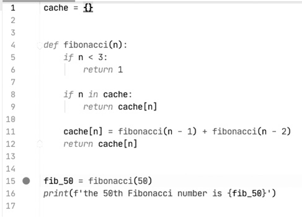
Figure 16: Setting a breakpoint in the code
To launch the Fibonacci run configuration in debug mode, instead of clicking the green play button, you want to click the red bug button (see Figure 15) or select Run ▸ Debug ‘fibonacci’ from the menu.
PyCharm launches our script and checks for breakpoints; as soon as it finds one, it stops execution before executing that line. Your IDE should’ve halted execution in the line where we set the breakpoint and displayed the debugger controls in the lower part, as in Figure 17.
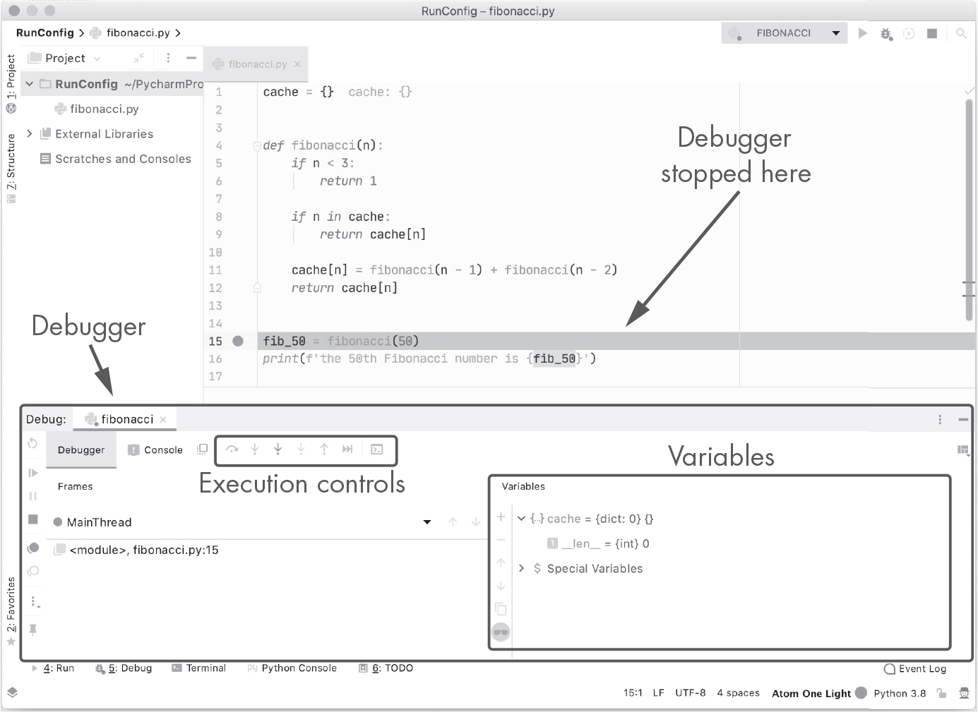
Figure 17: PyCharm’s debugger
The debugger has a bar near the top to control the execution of the program (see Figure 18). There are a few icons, but we’re mainly interested in the first two: Step over and Step into. With the Step over option, we can execute the current line and jump to the next one. The Step into option goes inside the function body of the current line. We’ll look at these two in a minute.
The right side of the debugger has a Variables pane where we can inspect the current state of our program: the values of all the existing variables. For instance, we can see the cache variable in Figure 17, which is an empty dictionary at the moment.

Figure 18: Debugger execution controls
Let’s now click the Step into icon in the execution control’s section of the debugger. The execution enters the fibonacci function body and stops in its first instruction (Figure 19).
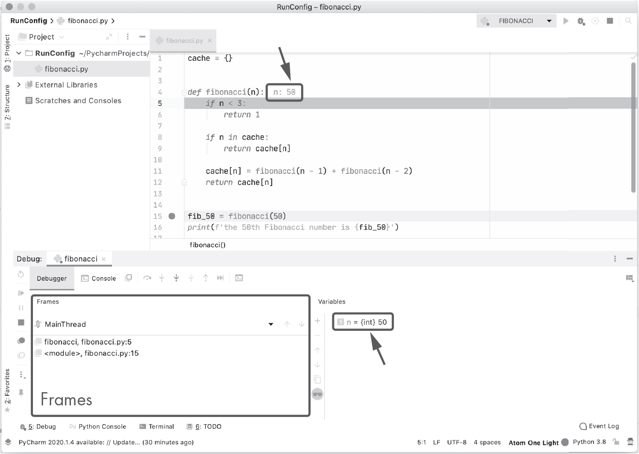
Figure 19: Stepping into the fibonacci function
The debugger’s Variables pane now shows the n variable with its current value, 50. This value also appears beside the fibonacci function definition, as you can see in Figure 19 (both places are indicated with arrows).
The left side of the debugger displays the Frames pane. This pane contains the stack frames of our program. Each time a function is executed, a new frame is pushed to the stack with the function’s local variables and some more information. You can go back and forth in time by clicking a frame to inspect the state of the program before that function got called. For instance, you can click the <module>, fibonacci.py:15 stack frame to go back in time before the fibonacci function got called. To go back to the current execution point, simply click the topmost stack frame, fibonacci, fibonacci.py:5 in this case.
Try to continue debugging the program using the Step over and Step into controls. Make sure you watch the cache and n variables as they change their values. Once you’re done experimenting, to stop the debugging session, you can either execute all the instructions in the program until it finishes or click the Stop button in the debugger. You can do this from the menu by selecting Run ▸ Stop ‘fibonacci’ or by clicking the red square icon on the left side of the debugger.
Let’s try one last debugging exercise. Run the program again in debug mode; when the execution stops at the breakpoint, click the Step over icon. Inspect the cache variable in the Variables pane. As you can see, the cache is now filled with all the Fibonacci numbers from 3 up to 50. You can expand the dictionary to check all of the values inside, as in Figure 20.
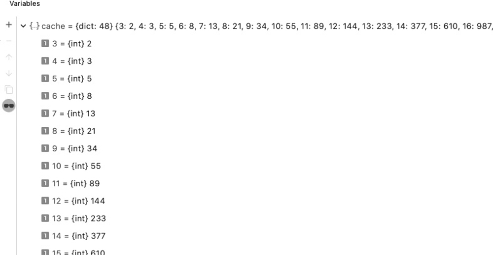
Figure 20: Debugger variables
You can also interact with the current status of the program using the debugger’s console (Figure 21). In the debugger view, click the Console tab next to the Debugger tab. In this console, you can interact with the state of the current program and do things like check whether a given Fibonacci number is cached:
>>> 12 in cache
True
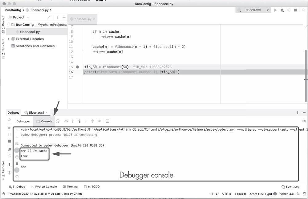
Figure 21: Debugger console
Summary
In this introductory chapter, we’ve taken a look at the contents of the book and the prerequisites you’ll need to follow along and make the best of it. We also installed Python and configured our environment to work effectively throughout the book.
The last section was a sneak peek into PyCharm and its powerful debugging tools, but as you can imagine, we’ve barely scratched the surface. To learn more about PyCharm debugging, take a quick look at the official documentation at https://www.jetbrains.com/help/pycharm/debugging-code.html.
Now, let’s start learning about Python.