
Video Tone Mapping
R. Boitard*,†; R. Cozot*; K. Bouatouch* * IRISA, Rennes, France
† Technicolor, Cesson-Sevigne, France
Abstract
To display high dynamic range videos on a low dynamic range display, a tone mapping operation is needed. Tone mapping independently each frame of a video sequence leads to temporal artifacts that impair the visual quality of the resulting tone-mapped video. These temporal artifacts are classified into six categories: global flickering, local flickering, temporal noise, temporal brightness incoherency, temporal object incoherency, and hue coherency. We explain in detail the situations in which these artifacts may occur. We review existing video tone mapping operators (techniques that take into account more than a single frame) and show which artifacts are handled by these operators.
Keywords
Video; High dynamic range; Tone mapping; Temporal coherence; Visual artifacts
Each pixel of a low dynamic range (LDR) image is stored as color components, usually three. The way LDR displays interpret these components to shape color is defined through a display-dependent color space — for example, BT.709 (ITU, 1998) or BT.2020 (ITU, 2012). In contrast, high dynamic range (HDR) pixels represent, in floating point values, the captured physical intensity of light in candelas per square meter. They can also represent relative floating point values. Hence, adapting an HDR image to an LDR display amounts to retargeting physical values, with a virtually unlimited bit depth, to a constrained space (22n chromaticity values over 2n tonal level, n being the targeted bit depth). This operation, which ensures backward compatibility between HDR content and LDR displays, is called tone mapping. The bit-depth limitation means that many similar HDR values will be tone-mapped to the same LDR value. Consequently, contrast between neighboring pixels as well as between spatially distant areas will be reduced. Furthermore, LDR displays have a low peak luminance value when compared with the luminance that a real scene can achieve. Consequently, captured color information will have to be reproduced at different luminance levels.
In a nutshell, tone mapping an HDR image amounts to finding a balance between the preservation of details, the spatial coherency of the scene, and the fidelity of reproduction. One usually achieves this balance by taking advantage of the many weaknesses of the human visual system. Furthermore, the reproduction of a scene can sometimes be constrained by an artist or application intent. That is why a lot of tone mapping operators (TMOs) have been designed with different intents, from simulating human vision to achieving the best subjective quality (Reinhard et al., 2010; Myszkowski et al., 2008; Banterle et al., 2011).
In the early 1990s, the main goal of tone mapping was to display computer-generated HDR images on a traditional display. Indeed, use of a simple gamma mapping was not enough to reproduce all the information embedded in HDR images. Although throughout the years TMOs addressed different types of applications, most of them still focused on finding the optimal subjective quality, as the many subjective evaluations attest (Drago et al., 2003; Kuang et al., 2007; Čadík et al., 2008). However, because of the lack of high-quality HDR video content, the temporal aspect of tone mapping has been dismissed for a long time. Thanks to recent developments in the HDR video acquisition field (Tocci et al., 2011; Kronander et al., 2013, 2014), more and more HDR video content is now becoming publicly available (Unger, 2013; Krawczyk, 2006; Digital Multimedia Laboratory, 2014; Lasserre et al., 2013; IRISA, 2015). Soon many applications such as real-time TV broadcasting, cinema movies, and user-generated videos will require video tone mapping.
In this chapter, we propose to evaluate the status of the video tone mapping field when trying to achieve a defined subjective quality level. Indeed, naively applying a TMO to each frame of an HDR video sequence leads to temporal artifacts. That is why we describe, in Section 6.1, different types of temporal artifacts found through experimentation. Then, Section 6.2 introduces state-of-the-art video TMOs — that is to say, TMOs that rely on information from frames other than the frame currently being tone-mapped. In Section 6.3, we present two new types of temporal artifact that are introduced by video TMOs: temporal contrast adaptation (TCA) and ghosting artifacts (GAs). Finally, Section 6.4 presents in more detail two recently published video TMOs.
6.1 Temporal Artifacts
Through experimentation with different HDR video sequences, we encountered several types of temporal artifact. In this section we focus only on those occurring when a TMO is applied naively to each frame of an HDR video sequence. We propose classifying these artifacts into six categories:
1. Global flickering artifacts (GFAs; Section 6.1.1),
2. Local flickering artifacts (LFAs; Section 6.1.2),
3. Temporal noise (Section 6.1.3),
4. Temporal brightness incoherency (TBI; Section 6.1.4),
5. Temporal object incoherency (TOI; Section 6.1.5),
6. Temporal hue incoherency (THI; Section 6.1.6).
This section provides a description of those artifacts along with some examples. Note that all the results are provided with TMOs that do not handle time dependency — namely, TMOs that rely only on statistics of the current frame for tone mapping.
6.1.1 Global Flickering Artifacts
GFAs are well known in the video tone mapping literature and are characterized by abrupt changes, in successive frames, of the overall brightness of a tone-mapped video sequence. These artifacts appear because TMOs adapt their mapping using image statistics that tend to be unstable over time. Analysis of the overall brightness of each frame over time is usually sufficient to detect those artifacts. An overall brightness metric can be, for example, the mean luma value of an image. Note that if it is computed on HDR images, the luminance channel must first be perceptually encoded, with use of, for example, a log transform as proposed in Reinhard et al. (2002), before averaging is done.
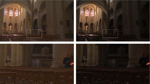
To illustrate this type of artifact, we plot in Fig. 6.1 the overall brightness indication for both the HDR sequence and the tone-mapped sequence. Note how the evolution of the overall brightness is stable over time in the HDR sequence, while abrupt peaks occur in the LDR sequence. These artifacts appear because one of the TMO’s parameters, which adapts to each frame, varies over time. Fig. 6.2 illustrates such an artifact occurring in two successive frames of a tone-mapped video sequence. The overall brightness has changed because the relative area of the sky in the second frame is smaller, hence reducing the chosen normalization factor (99th percentile).


To summarize, GFAs mostly occur when one is using TMOs that rely on content-adaptive parameters that are unstable over time. They are usually considered as the most disturbing of the artifacts presented in this section, which is why they have received a lot of attention, as will be seen in Section 6.2.
6.1.2 Local Flickering Artifacts
LFAs correspond to the same phenomenon as their global counterpart but on a reduced area. They appear mostly when one is using TMOs that map a pixel on the basis of its neighborhood — namely, local TMOs. Small changes of this neighborhood, in consecutive frames, may result in a different mapping. Edge-aware TMOs are particularly prone to such artifacts as they decompose an HDR image into a base layer and one or more detail layers. As each layer is tone-mapped independently, a difference in the filtering in successive frames results in LFAs.
The top row in Fig. 6.3 represents a zoom on a portion of the computed base layer of three successive frames. Note how the edges are less filtered out in the middle frame compared with the other two frames. Application of the bilateral filter (Durand and Dorsey, 2002) operator results in an LFA in the tone-mapped result (bottom row). Although LFAs are visible in a video sequence, it is tenuous to represent LFAs by means of successive frames. A side effect of LFAs is that they modify the saliency of the tone-mapped sequence as the eye is attracted by these changes of brightness on small areas.

6.1.3 Temporal Noise
Temporal noise is a common artifact occurring in digital video sequences. Noise in digital imaging is mostly due to the camera and is particularly noticeable in low-light conditions. On images, camera noise has a small impact on the subjective quality; however, for video sequences its variation over time makes it more noticeable. This is why denoising algorithms (Brailean et al., 1995) are commonly applied to video sequences to increase their subjective quality.
As most TMOs aim to reproduce minute details, they struggle to distinguish information from noise. Consequently, most current TMOs increase the noise rather than reducing it. Local TMOs are particularly prone to such artifacts as they aim to preserve details even in dark areas, which tend to be quite noisy. Furthermore, noise is usually reproduced at a luma level higher than that of a native LDR image, which makes the noise more visible. An example of temporal noise enhanced by the application of local TMOs is illustrated in Fig. 6.4.
6.1.4 Temporal Brightness Incoherency
TBI artifacts occur when the relative brightness between two frames of an HDR sequence is not preserved during the tone mapping. As a TMO uses for each frame all its available range, the temporal brightness relationship between frames is not preserved throughout the tone mapping operation. Consequently, a frame perceived as the brightest in the HDR sequence is not necessarily the brightest in the LDR sequence.
For example, TBI artifacts occur when a change of illumination condition in the HDR sequence is not preserved during the tone mapping. Consequently, temporal information (ie, the change of condition) is lost, which changes the perception of the scene (along with its artistic intent). Fig. 6.5 illustrates a TBI artifact, where the overall brightness of both the HDR sequence and the LDR sequence is plotted. Note that although the mean value varies greatly in the HDR sequence, it remains stable in the LDR one. This is because a TMO searches for the best exposure for each frame. As it has no information on temporally close frames, the change of illumination is simply dismissed and the best exposure is defined independently (usually in the middle of the available range). Fig. 6.6 illustrates an example of TBI occurring in consecutive frames of a tone-mapped video sequence. The top row displays the HDR luminance of these frames in false color. The change of illumination conditions occurs when the disco ball light source is turned off. When a TMO is applied, this change of illumination condition is lost (bottom row).


TBI artifacts can appear even if no change of illumination condition occurs — that is to say, when the tone mapping adapts to the content. When this adaptation occurs abruptly on successive frames, it gives rise to flickering artifacts as seen previously. However, when this adaptation is smoother — say, over a longer time — the brightness relationship between the HDR and LDR sequences will be slowly disrupted. These artifacts are similar to those that occur when commercial cameras adapt their exposure during a recording (Farbman and Lischinski, 2011). Such an artifact is shown in Fig. 6.7 as the brightest HDR frame (rightmost) is the dimmest one in the LDR sequence. This second cause of TBI artifacts is also a common cause of TOI, which is presented next.

6.1.5 Temporal Object Incoherency
TOI occurs when an object’s brightness, stable in the HDR sequence, varies in the LDR sequence. Fig. 6.8 plots the HDR and LDR overall brightness along with the value of a single pixel over several frames. Note that the HDR pixel’s value is constant over time, while the overall brightness changes. As the TMO adapts to each frame, the LDR pixel’s value changes, resulting in a TOI artifact. Fig. 6.7 illustrates visually such an artifact. When looking at the false color representation of the HDR luminance (Fig. 6.7, top row), one sees the level of brightness of the underside of the bridge to be stable over time. However, after application of a TMO (bottom row), the bridge, which appears relatively bright at the beginning of the sequence, is almost dark at the end. The temporal coherency of the bridge in the HDR sequence has not been preserved in the LDR sequence. The adaptation of a TMO to a scene is the source of TBI and TOI artifacts. However, TBI artifacts are of a global nature (difference in overall brightness between frames), while TOI artifacts are of a local nature (difference in brightness between a reduced area over time).

6.1.6 Temporal Hue Incoherency
THI is closely related to TBI as it corresponds to the variation of the color perception of an object rather than its brightness. Such artifacts occur when the balance between tristimulus values in successive frames is not temporally preserved by the tone mapping. The main reason for this imbalance is color clipping. Color clipping corresponds to the saturation of one or more of the tone-mapped color channels (eg, red, green, or blue). Color clipping is a common artifact inherent in tone mapping of still images when one aims to reproduce as well as possible the HDR color (Xu et al., 2011; Pouli et al., 2013). When color clipping is considered as a temporal artifact, it is not the difference between the HDR and LDR reproduction that is important but rather the LDR coherency from frame to frame. Indeed, variations in the tone mapping may saturate one color channel of an area which was not in the previous frame.
To illustrate such an artifact, we generated an HDR sequence with the following characteristics:
• A square area of constant luminance (100 cd/m2) with two gradients along the CIE u![]() and v
and v![]() chrominances. The chrominance gradient ranges from −0.25 to 0.25 around the D65 white point.
chrominances. The chrominance gradient ranges from −0.25 to 0.25 around the D65 white point.
• A neutral gray border area with a temporally varying luminance ranging from 0.005 to 10,000 cd/m2.
Fig. 6.9 illustrates a THI due to the clipping of one or more color channels by a TMO. Note the shift in hue illustrated both in Fig. 6.9A (right) and in a zoom on a portion of the tone-mapped frames (Fig. 6.9B).

6.2 Video TMOs
Applying a TMO naively to each frame of a video sequence leads to temporal artifacts. The aim of video TMOs is to prevent or reduce those artifacts. Video TMOs rely on information outside the current frame to perform their mapping. Most current video TMOs extend or postprocess TMOs designed for still images. We have sorted these techniques into three categories depending on the type of filtering:
1. Global temporal filtering (Section 6.2.1),
2. Local temporal filtering (Section 6.2.2),
3. Iterative filtering (Section 6.2.3).
For each category, we provide a description of the general technique along with different state-of-the-art references.
6.2.1 Global Temporal Filtering
Global temporal filtering aims to reduce GFAs when global TMOs are used. Indeed, global operators compute a monotonously increasing tone mapping curve that usually adapts to the image statistics of the frame to be tone-mapped. However, abrupt changes of this curve in successive frames result in GFAs. Two main approaches have been formulated so far to reduce those artifacts: filtering temporally either the tone mapping curve or the image statistics.
By application of a temporal filter to successive tone mapping curves, GFAs can be reduced. Such tone mapping curves are usually filtered during a second pass as a first pass is required to compute a tone mapping curve per frame. The display adaptive operator (Mantiuk et al., 2008) is able to perform such temporal filtering on the nodes of a computed piecewise tone mapping curve. The efficiency of this filtering is illustrated in Fig. 6.10. The top row provides the independently tone-mapped version of three successive frames of an HDR video sequence. The second row displays the corresponding piecewise tone mapping curves on top of their histogram. Note how the tone mapping curve of the middle frame is different from the other two, resulting in a change of overall brightness (GFA) in the tone-mapped result. The third row shows the temporally filtered version of the piecewise tone mapping curves. Finally, the bottom row provides the tone-mapped frames after the GFA has been reduced.

Image statistics can be unstable over time (eg, the 99th percentile, mean value, histogram of the luminance (Ward, 1994), etc.). For example, the photographic tone reproduction operator (Reinhard et al., 2002) relies on the geometric mean of an HDR image to scale it to the best exposure. One temporal extension of this operator filters this statistic along a set of previous frames (Kang et al., 2003). As a consequence, this method smooths abrupt variations of the frame geometric mean throughout the video sequence. This technique is capable of reducing flickering for sequences with slow illumination variations. However, for high variations it fails because it considers a fixed number of previous frames. That is why, Ramsey et al. (2004) proposed a method that adapts this number dynamically. The adaptation process depends on the variation of the current frame key value and that of the previous frame. Moreover, the adaptation discards outliers using a min/max threshold. This solution performs better than that of Kang et al. (2003) and for a wider range of video sequences. The computed geometric mean for these techniques and the original algorithm are plotted in Fig. 6.11. The green curve (Kang et al., 2003) smooths every peak but also propagates the resulting smoothed peaks to successive computed key values. The red curve (Ramsey et al., 2004), however, reduces the abrupt changes of the key value without propagating it to successive frames.

Another temporal extension of the photographic tone reproduction operator was proposed in Kiser et al. (2012). The temporal filtering consists of a leaky integrator applied to three variables (a, A, and B) that modify the scaling of the HDR frame:
where ![]() and
and ![]() , where
, where ![]() and
and ![]() are the maximum and minimum values of Lw, which is the HDR luminance. k corresponds to the geometric mean and the leaky integrator is computed as
are the maximum and minimum values of Lw, which is the HDR luminance. k corresponds to the geometric mean and the leaky integrator is computed as
where vt represents any of the three variables a, A, and B at time t and αv is a time constant giving the strength (leakiness) of the temporal filtering.
Many other TMOs filter their parameters temporally, including those in Pattanaik et al. (2000), Durand and Dorsey (2000), Irawan et al. (2005), and Van Hateren (2006). Most of them aim either to simulate the temporal adaptation of the human visual system or to reduce GFAs.
6.2.2 Local Temporal Filtering
Local temporal filtering consists in performing a pixelwise temporal filtering with or without motion compensation. Indeed, global temporal filtering cannot apply to local TMOs as such operators rely on a spatially varying mapping function. As outlined previously, local changes in a spatial neighborhood cause LFAs. To prevent these local variations of the mapping along successive frames, video TMOs can rely on pixelwise temporal filtering. For example, the gradient domain compression operator (Fattal et al., 2002) has been extended by Lee and Kim (2007) to cope with videos. This TMO computes an LDR result by finding the output image whose gradient field is the closest to a modified gradient field. Lee and Kim (2007) proposed adding a regularization term which includes a temporal coherency relying on a motion estimation:
where Ld is the output LDR luma at the preceding or current frame (t − 1 or t) and G is the modified gradient field. The pairs (x, y) and (δx, δy) represent, respectively, the pixel location of a considered pixel and its associated motion vectors. The parameter λ balances the distortion to the modified gradient field and to the previous tone-mapped frame.
Another operator (local model of eye adaptation (Ledda et al., 2004)) performs a pixelwise temporal filtering. However, the goal of this operator is to simulate the temporal adaptation of the human eye on a per-pixel basis. Besides increasing the temporal coherency, pixelwise temporal filtering also has denoising properties. Indeed, many denoising operators rely on temporal filtering to reduce noise (Brailean et al., 1995). Performing such a filtering during the tone mapping allows one to keep the noise level relatively low.
6.2.3 Iterative Filtering
The techniques presented so far in this section focus on preventing temporal artifacts (mostly flickering) when one is tone mapping video sequences. These a priori approaches consist in either preprocessing parameters or modifying the TMO to include a temporal filtering step. Another trend analyzes a posteriori the output of a TMO to detect and reduce temporal artifacts, the reduction consisting in iterative filtering.
One of these techniques (Guthier et al., 2011) aims at reducing GFAs. Such an artifact is detected if the overall brightness difference between two successive frames of a video sequence is greater than a brightness threshold (defined with either Weber’s law (Ferwerda, 2001) or Steven’s power law (Stevens and Stevens, 1963)). As soon as an artifact is located, it is reduced by an iterative brightness adjustment until the chosen brightness threshold is reached. Note that this technique performs an iterative brightness adjustment on the unquantized luma to avoid loss of signal due to clipping and quantization. Consequently, the TMO’s implementation needs to embed and apply the iterative filter before the quantization step. This technique relies only on the output of a TMO and hence can be applied to any TMO. Fig. 6.12 illustrates the reduction of a GFA when this postprocessing is applied.

6.3 Temporal Artifacts Caused by Video TMOs
In the previous section, we presented solutions to reduce temporal artifacts when one is performing video tone mapping. These techniques target mostly flickering artifacts as they are considered as one of the most disturbing artifacts. However, these techniques can generate two new types of temporal artifact — temporal contrast adaptation (TCA) and ghosting artifacts (GAs) — which we describe in this section.
6.3.1 Temporal Contrast Adaptation
To reduce GFAs, many TMOs rely on global temporal filtering. Depending on the TMO used, the filter is either applied to the computed tone mapping curve (Mantiuk et al., 2008) or to the parameter that adapts the mapping to the image (Ramsey et al., 2004; Kiser et al., 2012). However, when a change of illumination occurs, as shown in Fig. 6.6, it also undergoes temporal filtering. Consequently, the resulting mapping does not correspond to any of the conditions but corresponds rather to a transition state. We refer to this artifact as temporal contrast adaptation (TCA). Fig. 6.13 illustrates the behavior of the temporal filtering when a change of illumination occurs. Note how the tone mapping curve, plotted on top of the histograms, shifts from the first illumination condition (frame 130) toward the second state of illumination (frame 150; see Fig. 6.6 for the false color luminance). As the tone mapping curve has anticipated this change of illumination, frames neighboring the change of illumination are tone-mapped incoherently.

These artifacts also occur when one is performing postprocessing to detect and reduce artifacts as in Guthier et al. (2011). Indeed, this technique relies only on the LDR results to detect and reduce artifacts. If one has no information related to the HDR video, then a change of illumination suppressed by a TMO cannot be anticipated or predicted.
6.3.2 Ghosting Artifacts
Similarly to global temporal filtering, local temporal filtering generates undesired temporal artifacts. Indeed, pixelwise temporal filtering relies on a motion field estimation which is not robust to a change of illumination conditions and object occlusions. When the motion model fails, the temporal filtering is computed along invalid motion trajectories, which results in GAs.
Fig. 6.14 illustrates a GA in two successive frames resulting from the application of the operator of Lee and Kim (2007). This artifact proves that pixelwise temporal filtering is efficient only for accurate motion vectors. A GA occurs when a motion vector associates pixels without a temporal relationship. Those “incoherent” motion vectors should be accounted for to prevent GAs, as these are the most disturbing artifacts (Eilertsen et al., 2013).

6.4 Recent Video TMOs
Recently, two novel contributions have been proposed in the field of video tone mapping. The first one, called zonal brightness coherency (ZBC) (Boitard et al., 2014), aims to reduce TBI and TOI artifacts through a postprocessing operation which relies on a video analysis performed before the tone mapping. The second one (Aydin et al., 2014) performs a ghost-free pixelwise spatiotemporal filtering to achieve high reproduction of contrast while preserving the temporal stability of the video.
6.4.1 Zonal Brightness Coherency
The ZBC algorithm (Boitard et al., 2014) aims to preserve the HDR relative brightness coherency between every object over the whole sequence. Effectively, it should reduce TBI, TOI, and TCA artifacts and in some cases THI artifacts. It is an iterative method based on the brightness coherency (Boitard et al., 2012) technique which considered only overall brightness coherency. This method consists of two steps: a video analysis and postprocessing.
The video analysis relies on a histogram-based segmentation as shown in Fig. 6.15. A first segmentation on a per frame basis provides several segments per frame. The geometric mean (called “key value” in the article) of each segment of each HDR frame is computed and used to build a second histogram, which is in turn segmented to compute zone boundaries. The key value kz(Lw) is computed for each zone of each frame. An anchor is then chosen either automatically or by the user to provide an intent for the rendering.

Once the video analysis has been performed, each frame is tone-mapped with any TMO. Then a scale ratio sz is applied to each pixel luminance Lm,z of each video zone z to ensure that the brightness ratio between the anchor and the current zone in the HDR sequence is preserved in the LDR sequence (Eq. 6.4):

where Lzbc,z is the scaled luminance, ζ is a user-defined parameter, kvz(Lw) is the anchor zone HDR key value, kvz(Lm) is the anchor zone LDR key value, kz(Lw) is the z zone HDR key value and kz(Lm) is the z zone LDR key value. Note that the subscript z stands for zone.
At the boundaries between two zones, an alpha blending is used to prevent abrupt spatial variations. The whole workflow of this technique is depicted in Fig. 6.16.

 . Their respective scaling ratios sj and sj,j+1 are computed. The ZoneScaling function applies the scale ratios to the tone-mapped frames. Finally, Q quantizes linearly floating point values in the range [0;1] to integer values on a defined bit depth n (values in the range [0;2n − 1]).
Fig. 6.17 presents some results obtained when ZBC postprocessing is used on tone-mapped video sequences where temporal artifacts occurred. The left plot provides results regarding the reduction of the TOI artifact that was illustrated in Fig. 6.8. Thanks to the ZBC technique, the value of the pixel, which was constant in the HDR sequence, is much stabler over time. Note also that the LDR mean value is quite low at the beginning of the sequence, which will most likely result in a loss of spatial contrast in the tone-mapped frames. That is why Boitard et al. (2014) have provided a user-defined parameter which effectively trades off temporal coherency for an increase in spatial reproduction capabilities (see ζ in Eq. 6.4). In the right plot, we show some results regarding the reduction of TBI artifacts. This plot is to be compared with the one in Fig. 6.5. Use of ZBC postprocessing on the Disco sequence allows the change of illumination present in the HDR sequence to be preserved.

More results are available in Boitard et al. (2014) and Boitard (2014), especially regarding the preservation of fade effects and the impact of the different parameters of this technique.
6.4.2 Temporally Coherent Local Tone Mapping
In Section 6.3.2, we explained why pixelwise temporal filtering can cause GAs. However, this type of filtering is the only known solution to prevent LFAs that can arise when local TMOs are used. Consequently, Aydin et al. (2014) proposed a spatial filtering process to ensure high reproduction of contrast when ghost-free pixelwise temporal filtering is performed. Fig. 6.18 illustrates the workflow of this technique.

This technique considers a temporal neighborhood composed of a center frame Ik and temporally close frames Ik ± i. In a first step, each frame is decomposed into a base and detail layer by use of a permeability map (spatial diffusion weights). Both subbands are then motion compensated (warped) with a previously computed motion flow. Note that no warping is necessary for the subbands associated with the central frame.
The second step consists of two temporal filters which allow separate filtering of the base and detail layers. To prevent GAs, the filtering relies on confidence weights composed of a photoconstancy permeability map and a penalization on pixels associated with high gradient flow vectors. The photoconstancy permeability map is computed between successive frames and corresponds to a temporal transposition of the spatial diffusion weight on which the spatial decomposition relies. Aydin et al. (2014) observed that this photoconstancy measure can be tuned to stop temporal filtering at most warping errors, hence preventing the appearance of GAs. However, it also defeats the purpose of temporal filtering, which is to smooth medium to low temporal variations. That is why the penalization term has been introduced as it is a good indication of complex motion where the flow estimation tends to be erroneous. This step provides two images, the spatiotemporally filtered base layer Bk and a temporally filtered detail layer Dk.
To obtain the tone-mapped frame ![]() , the base layer Bk can be fed to any TMO and then combined with the detail layer Dk, a process similar to that detailed in Durand and Dorsey (2002). This method addresses several of the artifacts presented in this chapter. First, the temporal noise is reduced as the details are filtered temporally. Second, LFAs are minimized thanks to the pixelwise temporal filtering. Finally, GAs are prevented by adaptation of the temporal filtering to a motion flow confidence metric. A simplified illustrative workflow is depicted in Fig. 6.19.
, the base layer Bk can be fed to any TMO and then combined with the detail layer Dk, a process similar to that detailed in Durand and Dorsey (2002). This method addresses several of the artifacts presented in this chapter. First, the temporal noise is reduced as the details are filtered temporally. Second, LFAs are minimized thanks to the pixelwise temporal filtering. Finally, GAs are prevented by adaptation of the temporal filtering to a motion flow confidence metric. A simplified illustrative workflow is depicted in Fig. 6.19.

As this technique is fairly new, extended results with more HDR sequences could help detect new types of artifacts. In particular, it would be interesting to test this method when changes of illumination or cut occur in a sequence. Furthermore, most of the results provided with this technique rely on user interaction to achieve the best trade-off between temporal and spatial contrast. This is not achievable for many applications, such as live broadcasts and tone mapping embedded in set-top boxes.
6.5 Summary
In this chapter, we have described known types of temporal artifact that occur when HDR video sequences are tone-mapped. We have categorized video TMOs with respect to how they handle temporal information, and we have shown that although these solutions can deal with certain types of temporal artifact, they can also be a source of new ones. An evaluation of video TMOs (Eilertsen et al., 2013) reported that none of the current solutions can handle a wide range of sequences. However, this study was performed before the publication of the two video TMOs presented in Section 6.4. These two techniques, albeit significantly different, provide solutions to types of artifact not dealt with before.
Table 6.1 gives an overview of the temporal artifacts presented in this chapter, along with possible solutions. From this table, we can see that all of the artifacts described in this chapter have a solution. However, none of the video TMOs presented here encompass all of the tools needed to deal with all different types of artifact. Furthermore, the appearance of more HDR video sequences and applications for video tone mapping will likely result in new types of temporal artifact. Although the two recent contributions have significantly advanced the field of video tone mapping, more work still lies ahead.
Table 6.1
Summary of Temporal Artifacts Along With Their Main Causes and Possible Solutions
| Temporal Artifact | Possible Cause | Possible Solutions |
| Global flicker | Temporal instability of parameters | Global temporal filtering |
| Local flicker | Different spatial filtering in successive frames | Pixelwise temporal filtering |
| Temporal noise | Camera noise | Spatial and/or temporal filtering (pixelwise) |
| TBI (brightness) | Change of illumination adaptation of the TMO | Brightness analysis of each frame |
| TOI (object) | Adaptation of the TMO | Brightness analysis per zone of frames |
| THI (hue) | Saturation of color channel (due to clipping) | Hue and brightness analysis per zone of frames |
| TCA (contrast) | Global temporal filtering | Brightness analysis per zone of frames |
| Ghosting | Pixelwise temporal filtering | Confidence weighting of pixelwise temporal filtering |