17.1 Introduction

In Chapter 16, the concept of quality of experience (QoE) was discussed and it was highlighted how high dynamic range (HDR) video processing can impact different aspects of HDR QoE. This chapter is devoted to the analysis of state-of-the-art objective methods for measuring the quality of HDR image and video, as part of evaluating one of the components in the overall QoE. First, we mention a few additional considerations in HDR video quality measurement. These include the following:

• HDR video compression may suffer from new distortions in addition to the low dynamic range (LDR) ones (eg, loss of details due to saturation from an inverse tone mapping operator in addition to blockiness). This calls for investigation of methods that can deal with the new situation.

• Traditional LDR rendering usually does not consider the display used because the format and specifications are more standardized. By contrast, HDR rendering will need to take into account the display used (ie, LDR or HDR display). Both displays would need specific preprocessing, which can introduce artifacts. As a result, there is a need to analyze and quantify the possible effects of display toward HDR content rendering.

• The loss of details due to distortions (arising from preprocessing, compression, transmission errors, and so on) is an issue in LDR imaging. This will remain in HDR imaging but with the additional consideration of the artistic intent of HDR content, which can be altered by different processing. This problem is potentially more prominent in HDR imaging as it focuses on incorporating very high contrasts.

We can elaborate on and explain the above points further by considering a simplified diagram of a typical HDR video delivery system as shown in Fig. 17.1.

As shown, there are three main blocks — namely, content generation, distribution, and rendering. The first block pertains to HDR content generation. This can be realized if the scene is captured with a camera (single shot or multiexposure fusion based) or content can be computer generated. The second and third blocks concern content distribution and rendering, respectively, and are the main focus of this chapter.

The goal of HDR video encoding is to reduce the number of stored or transmitted bits. A video encoder exploits both temporal and spatial redundancies in the video signal to compress it. However, this inevitably leads to loss of visual quality and the encoder always needs to deal with a trade-off between data reduction and visual quality. Similarly, video quality measurement is required toward the optimal design of transmission system parameters so that the end user receives at least acceptable-quality content.

For content rendering, postprocessing is also usually applied to maintain or enhance visual quality. Finally, one needs to measure the impact of display-specific processing on the rendered HDR video. In our context, we can consider either HDR or LDR displays. Even an HDR display needs to preprocess (tone map) video data so that the maximum displayable luminance¹ is not exceeded. On the other hand, LDR displays as such cannot provide high luminance conditions and thus require tone-mapped content for rendering. However, tone mapping is known to be a nontransparent operation which can reduce the levels of details as well as modify artistic intent (Narwaria et al., 2014b). Thus, quality measurement is an important aspect all along the HDR delivery chain, and we have highlighted a few scenarios for it.

The HDR processing chain entails that distortion might appear in new forms, even when it was not present or visible in analog LDR circumstances. For instance, consider the LDR image in Fig. 17.2A. The luminance of the scene was rather low; thus, the picture contains noise in the dark regions. However, when the image is displayed on a standard dynamic range display, this noise is hardly visible in dark areas at the bottom of the picture and the quality of the image is high. Fig. 17.2B shows the result of expanding the dynamic range of this image to match that of an HDR display (the result has been tone-mapped for this illustration). The inverse tone mapping algorithm is the linear expansion described in Akyüz et al. (2007). Although an HDR reproduction device is necessary to appreciate the content of this picture, the tone-mapped version in Fig. 17.2B clearly shows that the noise in the dark regions is boosted to a visible level. This example illustrates that perceived distortion can be significantly affected by the HDR processing chain.

Other examples of HDR-specific distortion are banding, due to a limited resolution of HDR encodings, and color changes due to the much wider gamut color provided by HDR. Finally, oversmoothing may happen in tone mapping-based HDR video compression (see Chapter 10 for a comprehensive treatment of this topic): areas where the original HDR frames contain details that are tone-mapped to very close LDR values might then be smoothed out by transform coding. As a result, these details will be lost after inverse tone mapping at the decoder.

As discussed in Chapter 16, the different aspects of HDR QoE (including video quality) can be measured by subjective and objective methods. The former involves the use of human subjects to judge and rate the quality of the test stimuli. With appropriate laboratory conditions and a sufficiently large subject panel, it remains the most accurate method. The latter quality assessment method uses a computational (mathematical) model to provide estimates of the subjective video quality. While such objective models may not mimic subjective opinions accurately in a general scenario, they can be reasonably effective in specific conditions/applications. Hence, they can be an important tool toward automating the testing and standardization of HDR video processing algorithms, especially when subjective tests may not be feasible. Therefore, this chapter deals with objective quality assessment of HDR content and elaborates on the issues and challenges that arise. We also discuss and present details of the existing efforts on the topic. Particularly, the focus is on full-reference HDR metrics which take as input two HDR signals (one of them is always assumed to be the reference). Hence, in the context of this chapter, the term “quality” can also be interpreted as “fidelity,” and both can be used interchangeably. Another use case is that of comparing HDR and LDR signals, and this is needed, for instance, when HDR content is tone-mapped to be rendered on an LDR display.

17.2 Approaches for Assessing HDR Fidelity

LDR pixel values are typically gamma encoded. As a consequence, LDR video encodes information that is nonlinearly (the nonlinearity arising from the gamma curve which can approximate the response of human eye to luminance) related to the scene luminance. This implies that the changes in LDR pixel values can be approximately linearly related to the actual change perceived by the human visual system (HVS). However, HDR pixel values are related (proportional) to the physical luminance. Hence, direct pixel-based differences (between reference and distorted HDR signals) may not be meaningful. This issue can tackled by two approaches. The first one is to explicitly model certain mechanisms of the HVS. The second approach is to transform the luminance values to a perceptually relevant space, and then use an LDR method for quality assessment (ie, adaptation of LDR metrics). The two approaches are briefly discussed next.

17.3 From Spatial Frequency Errors to Global Quality Measure of HDR Content: Improvement of the HVS-Based Model

In Section 17.2.1 we briefly described the HDR-VDP-2 method, and outlined the need to obtain the pooling weights for errors in different frequency bands. In the original implementation of HDR-VDP-2, the pooling weights were determined by optimization on an existing LDR dataset. There are, however, three limitations of that approach, especially in the context of dealing with LDR and HDR conditions. First, Mantiuk et al. (2011) used only an LDR image quality dataset, which did not include any HDR images. Second, the optimization was done on a relatively small number of images. Finally, because the optimization was unconstrained, it lead to negative pooling weights that may not be easily interpretable. These limitations were addressed by Narwaria et al. (2015a) in HDR-VDP-2.2, which was built upon HDR-VDP-2.

In HDR-VDP-2, the following expression is used to predict the quality score Q_HDRVDP for a distorted image with respect to its reference:

$\begin{array}{l}\hfill Q_{\text{HDRVDP}}=\frac{1}{F\cdot O}\sum _{f=1}^F\sum _{o=1}^O{\mathbf{w}}_{f}log\left(\frac{1}{I}\sum _{i=1}^I{\mathbf{D}}_{\text{p}}^2[f,o](i)+\epsilon \right),\end{array}$

where i is the pixel index, D_p denotes the noise-normalized difference between the fth spatial frequency (f = 1 to F) band and the oth orientation (o = 1 to O) of the steerable pyramid for the reference and test images, ε = 10⁻⁵ is a constant to avoid singularities when D_p is close to 0, and I is the total number of pixels. In the above expression, w_f is the vector of per-band pooling weights, which one can determine by maximizing correlations with subjective opinion scores. However, unconstrained optimization in this case may lead to some negative w_f. Because w_f determines the weight (importance) of each frequency band, a negative w_f is implausible and may indicate overfitting. Therefore, a constraint is introduced on w_f during optimization.

Let Q_HDRVDP and S, respectively, denote the vector of objective quality scores from HDR-VDP-2 and the vector of subjective scores for a given set of N images. Then the aim is to maximize the Spearman rank-order correlation between the two vectors, with w_f being the optimized variables. To that end, we first rank the values in Q_HDRVDP and S from 1 to N and obtain new vectors R_HDRVDP and R_subjective, which consist of the respective ranks. Further, we define E =R_HDRVDP −R_subjective as the rank difference vector. Then, the optimization problem can be formulated as

$\begin{array}{l}\hfill \underset{{\mathbf{w}}_f}{\text{Maximize}}\left(1-\frac{6\sum _{i=1}^N{\mathbf{E}}_i^2}{N(N^2-1)}\right),\text{subject to}{\mathbf{w}}_f\ge 0.\end{array}$

Also note that in this case the optimization can be solved by the Nelder-Mead method, which does not require the computation of gradients. This is because the objective function is not continuous and differentiable as Spearman rank-order correlation is used. Because the aim was to calibrate the metric so that it can handle both HDR and LDR conditions, Narwaria et al. (2015a) optimized w_f on the basis of a set of subjectively rated LDR and HDR images. The details of the HDR datasets can be found in Narwaria et al. (2013, 2014a), while the LDR datasets (TID2008 and CSIQ) were developed by Ponomarenko et al. (2008) and Larson and Chandler (2010).

17.3.1 Cross-Validation Results and Analysis

As reported by Narwaria et al. (2015a), there were 65 source content in total and 2932 distorted content (obtained by the application of different distortion types and levels to the source content). For the cross-validation studies, all the distorted images from 45 source contents was selected as the training set to find the optimal w_f vector, and the remaining images from 20 source content were used as a test set. To enable a more robust estimate of the prediction performance, the division into training and test sets was randomly repeated over 1000 iterations, and it was ensured that the two sets were different in terms of the source content. Hence, in each of the 1000 iterations, the prediction performance was assessed only for untrained content, thus providing a reasonably robust approach toward content-independent verification. With this data partition (45 source contents as the training set and remaining source contents as the test set), there were an average of 2032 and 900 images, respectively, in the training and test sets during each iteration.

The experimental results are shown in Fig. 17.3 (the bars from left to right correspond to the key entries from first to last), where the performance is measured in terms of mean (over 1000 iterations) values of Pearson and Spearman correlation values (a higher value implies better performance for these measures). One can see that the prediction performance with the weights obtained from the training set is better than that with the default weights as well as that of the two modified LDR methods. The 95% confidence intervals are also shown in Fig. 17.3 (denoted by error bars) to provide an indication of uncertainty in the measured values. As can be seen, the confidence intervals do not overlap, indicating a better performance with the trained weights from statistical considerations.

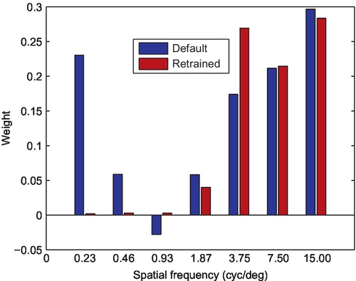
Finally, the retrained and default weights are compared via the frequency versus weight plot shown in Fig. 17.4. The frequency is expressed in cycles per degree and the left and right bars at each special frequency indicate default and retrained weights, respectively. The retrained weights reduce the importance of low-frequency bands. However, they are not necessarily related to the contrast sensitivity function because the goal of pooling is to quantify quality (or the annoyance level), which might not always be at the level of visibility thresholds. Also note that the negative weights found in the original HDR-VDP-2 could cause an increase of quality with a higher amount of distortion. This situation is valid only in very specific cases such as denoising and contrast enhancement (where visual quality may be enhanced). However, because this condition is not included in any of the datasets that we used, the retrained weights result in better physical interpretability (because all of them are positive, quality will decrease with increased level of distortion).

17.4 Adapted LDR Metrics for Measuring HDR Image Quality in the Context of Compression

This section provides a comparative analysis of the performance of adapted LDR metrics on compressed HDR images. The study was conducted by Valenzise et al. (2014), and the dataset used by them is publicly available for downloading.²

17.4.2 Dataset Description

Five HDR images were used, and these are shown in Fig. 17.5. These were taken from the HDR Photographic Survey dataset (Fairchild, 2007) in such a way to span a wide range of diverse content-specific characteristics, including spatial information, dynamic range, and overall brightness. All the selected images were adapted to the display resolution of 1920 × 1080 pixels. The test material was produced by compression of the source (reference) images with different codecs and coding conditions. In particular, three codecs were considered for test material generation: (a) JPEG; (b) JPEG 2000; (c) JPEG XT (Richter, 2013), which is the new standardization initiative (ISO/IEC 18477) of JPEG for backward-compatible encoding of HDR images. The HDR images were displayed on a SIM2 HDR47 display (SIM2, 2014), which has HD1080 resolution with a declared contrast ratio higher than 4×10⁶:1 and a maximum luminance of approximately 4250 cd/m². The subjective quality evaluation was performed following the double stimulus impairment scale method (ITU-R, 2012). Particularly, pairs of images (ie, the original image and the compressed image) were sequentially presented to the user, who was told that the first image was the reference and asked to rate the level of annoyance of the visual defects that she/he may observe in the second stimulus using a continuous quality scale ranging from 0 to 100, associated with five distinct descriptions (“very annoying,” “annoying,” “slightly annoying,” “perceptible,” and “imperceptible”). The pairs of stimuli were presented in random order, different for each viewer, with the constraint that no consecutive pairs concerning the same content will occur. More details on the experimental results can be found in Valenzise et al. (2014).

17.4.3 Results and Analysis

The subjective data (collected from 15 observers) were processed to compute the mean opinion score and the 95% confidence interval, assuming that the scores are following a Student’s t distribution.

The performance of the metrics was evaluated in terms of the Spearman rank-order correlation coefficient, computed on the entire set of mean opinion scores. The use of a nonparametric correlation coefficient avoids the need for nonlinear fitting to linearize the values of the objective metrics, which may be questionable because of the relatively small size of the subjective ground truth dataset. The values of the modulus of the correlation coefficient for each metric, per content and per codec, are reported in Table 17.1. Fig. 17.6 summarizes the performance of the metrics and shows also the 95% confidence interval of the Spearman correlation coefficient (modulus). As can be seen, overall the best performing LDR metric is PU-SSIM, followed by log SSIM. We also report results for HDR-VDP-2.1 and HDR-VDP-2.2, with the latter improving significantly over the older version of the metric, as discussed in the previous section. Interestingly, PU-SSIM has performance almost equivalent to that of HDR-VDP-2.2, albeit at lower computational cost.

Table 17.1

Spearman Correlation Coefficients (Modulus) Calculated for Each Content and Codec, With Maximum Correlation Values for Each Column Highlighted in Bold

	Overall	“Air Bellows Gap”	“Las Vegas Store”	“Mason Lake(1)”	“Redwood Sunset”	“Upheaval Dome”	JPEG	JPEG XT	JPEG 2000
PU-PSNR	0.794	0.976	0.963	0.976	0.952	0.987	0.591	0.797	0.835
PU-SSIM	0.923	0.952	1	0.952	1	0.975	0.942	0.944	0.887
log PSNR	0.866	0.976	0.963	0.976	0.976	0.987	0.753	0.832	0.887
log SSIM	0.904	0.952	0.975	0.928	0.952	0.975	0.907	0.881	0.872
HDR-VDP-2.1	0.889	0.952	0.987	0.976	0.952	0.987	0.802	0.909	0.924
HDR-VDP-2.2	0.946	0.929	0.985	0.952	0.970	1	0.942	0.927	0.958

In terms of content dependency and distortion dependency, these results confirm widely known observations concerning the scope of validity of most objective metrics (Huynh-Thu and Ghanbari, 2008). On one hand, the codec-dependent results show that all the metrics suffer to some extent from content dependency in their prediction capability. On the other hand, the content-dependent results clearly indicate that even perfect (ranking) prediction is reachable for some contents (ie, the results of PU-SSIM for content “LasVegasStore” and “RedwoodSunset”). Of course, one must interpret these results by taking into account the limited set of distortions which characterize the test database. Finally, it is interesting to notice that the range of PSNRs obtained in this work is significantly greater than that commonly encountered in the case of LDR image compression, as reported, for example, by De Simone et al. (2011).

17.5 Tone Mapping and Dynamic Range-Independent Metrics

In the previous sections, we discussed objective quality prediction of HDR content. Recall that in this approach it is assumed that both reference and distorted images have a similar dynamic range (hence, they can be either scene referred or display referred). However, there are many situations in which HDR video needs to be tone-mapped for it to be displayed on a typical LDR display, and this is where dynamic range-independent metrics can be useful.

We begin with the fact that tone mapping inherently produces images that are different from the original HDR reference. To fit the resulting image within the available color gamut and dynamic range of a display, tone mapping often needs to compress contrast and adjust brightness. A tone-mapped image may lose some quality as compared with the original seen on an HDR display, yet the images often look very similar and the degradation of quality is poorly predicted by most quality metrics. Smith et al. (2006) proposed the first metric intended for prediction of loss of quality due to local and global contrast distortion introduced by tone mapping. However, the metric was used only in the context of controlling a countershading algorithm and was not validated against experimental data. Aydın et al. (2008) proposed a metric for comparing HDR and tone-mapped images that is robust to contrast changes. The metric was later extended to video (Aydın et al., 2010). Both metrics are invariant to the change of contrast magnitude as long as that change does not distort contrast (reverse its polarity) or affect its visibility. The metric classifies distortions into three types: loss of visible contrast, amplification of invisible contrast, and contrast reversal. All three cases are illustrated in Fig. 17.7 for the example of a simple 2D Gabor patch. These three cases are believed to affect the quality of tone-mapped images. Fig. 17.8 shows the metric predictions for three tone-mapped images. The main weakness of this metric is that the distortion maps produced are suitable mostly for visual inspection and qualitative evaluation. The metric does not produce a single-valued quality estimate and its correlation with subjective quality assessment has not been verified. The metric can be conveniently executed from a Web-based service available at http://drim.mpi-sb.mpg.de/.

Yeganeh and Wang (2013) proposed a metric for tone mapping which was designed to predict the overall quality of a tone-mapped image with respect to an HDR reference. The first component of the metric is the modification of the SSIM index proposed by Wang et al. (2004), which includes the contrast and structure components, but does not include the luminance component. The contrast component is further modified to detect only the cases in which invisible contrast becomes visible and visible contrast becomes invisible, in a spirit similar to that in the dynamic range-independent metric of Aydın et al. (2008) described above. This is achieved by the mapping of local standard deviation values used in the contrast component into detection probabilities by a visual model, which consists of a psychometric function and a contrast sensitivity function. The second component of the metric describes “naturalness.” The naturalness is captured by the measure of similarity between the histogram of a tone-mapped image and the distribution of histograms from the database of 3000 LDR images. The histogram is approximated by the Gaussian distribution. Then, its mean and standard deviation are compared against the database of histograms. When both values are likely to be found in the database, the image is considered natural and is assigned a higher quality. The metric was tested and cross-validated with three databases, including one from Cadík et al. (2008) and the authors’ own measurements. The Spearman rank-order correlation coefficient between the metric predictions and the subjective data was approximately 0.8. Such a value is close to the value for a random observer, which is estimated as the correlation between the mean and random observer’s quality assessment.

An objective method for finding the optimal parameter space toward HDR tone mapping was proposed by Krasula et al. (2015). The method was aimed at addressing the nontrivial issue of proper tone mapping operator parameter selection because tone mapping operators usually need content-specific parameters in order to produce sharp and perceptually appealing pictures. It works by computing the percentage of area covered in a tone-mapped image. In the context of this method, the percentage of area covered can be used as an indicator of saturated and/or underexposed pixels. Hence, the method attempts to find a parameter space where the percentage is minimized. The method can be potentially applied in HDR content rendering and also security-related applications as suggested by Krasula et al. (2015). Fig. 17.9 provides an example to illustrate the concept of percentage of area covered. The two images in the top row were obtained with two different settings of a simple linear tone mapping operator, leading to images that will have different levels of details (it can be seen that the image on the right in the top row has more visible details). The maps (obtained on the basis of gradient and subsequent thresholding) shown below the corresponding images indicate areas where loss of details occurs because of very low (dark, shown in black) or very high (bright, shown in white) luminance, and the corresponding percentages of such areas (these are computed on the basis of the number of such overexposed/underexposed pixels and the total number of pixels in the image) are also indicated. The percentage of area covered will be equal to the sum of the percentages of the bright and dark areas. Obviously, a higher percentage of area covered will lead to loss of more details, and hence the concept can be used to tune tone mapping operator parameters to maximize the visibility of details in tone-mapped HDR content.

17.6 Extensions to Video

The previous sections discussed approaches for predicting quality in HDR images, and these can obviously be applied in the case of HDR video by applying them on frame-by-frame basis. However, this ignores the effect of temporal factors, which are also important for video quality measurement. Also note that application of HDR-VDP-2.2 for video can be computationally expensive because of the design of the metric. Therefore, this section discusses a method for objective measurement of HDR video quality proposed by Narwaria et al. (2015b), and has lower computational complexity. It is referred to as HDR-VQM and is based on PU encoding (recall this is one way of adapting a metric as discussed in Section 17.4). However, unlike image-based methods, HDR-VQM computes local quality considering spatiotemporal regions, and applies short-term and long-term pooling to derive the global quality score. Hence, it adopts true temporal pooling in contrast to image-based methods such as HDR-VDP-2.2.

17.6.1 Brief Description of HDR-VQM

A block diagram outlining the major steps in HDR-VQM is shown in Fig. 17.10. HDR-VQM takes as input the source and the distorted HDR video sequences. As shown in Fig. 17.10, the first two steps are meant to convert the native input luminance to perceived luminance. These can therefore be seen as preprocessing steps, and the first step is performed if the user provides emitted luminance values. Next, the impact of distortions is analyzed by comparison of the different frequencies and orientation subbands in the source (reference video sequence) and the hypothetical reference circuit (distorted video sequence). The last step is that of error pooling, which is achieved via spatiotemporal processing of the subband errors. This comprises short-term temporal pooling, spatial pooling, and finally, a long-term pooling. A separate block diagram explaining the error pooling in HDR-VQM is shown in Fig. 17.11.

As seen from Fig. 17.10, the first step is to convert native HDR values to display-referred luminance. Such a step is required because distortion visibility can be affected by the processing adopted to display HDR video. The second step is to convert the resulting luminance to perceived values (this approach was discussed in Section 17.2.2). Next, frequency domain filtering is used to obtain the subband errors. The subband error signal is then further processed via error pooling, which is elaborated in Fig. 17.11. It basically comprises short-term temporal pooling, which aims to pool or fuse the data in local spatiotemporal neighborhoods. This is followed by spatial pooling, which results in short-term quality scores, which can be seen as indicators of temporal quality. The final step uses a long-term temporal pooling in order to pool the short-term quality measures into a global video quality score. The reader is referred to Narwaria et al. (2015b) for more detailed discussions on the HDR-VQM formulation. We now compare the performance of HDR-VQM with that of other objective methods, including the adapted metrics and HDR-VDP-2.2.

17.6.2 Prediction Performance Comparison

The performance of HDR-VQM was analyzed on an HDR video dataset with a total of 90 HDR videos. These were obtained by compression of 10 source HDR sequences with a backward-compatible HDR video compression scheme. More details on dataset development can be found in Narwaria et al. (2015b).

A comparison of Pearson and Spearman correlation coefficients of different methods is shown in Fig. 17.12 (the bars from left to right correspond to the key entries from first to last), from which one can see that HDR-VQM performs better. The 95% confidence intervals for these correlation values are indicated by the error bars. Note that SSIM and PSNR were computed on PU-encoded values (hence these are referred to as P-SSIM and P-PSNR in Fig. 17.12). With regard to the computational complexity,⁴Fig. 17.13 provides the percentage of outliers and the relative computational complexity (expressed as the execution time relative to relative PSNR). Obviously, lower values for an objective method along both axes imply that it is better. It can be seen that the relative execution time for HDR-VQM is reasonable considering the improvements (ie, smallest percentage of outliers) in performance over the other methods. More specifically, as reported by Narwaria et al. (2015b), HDR-VQM (Linux cluster, 32 GB RAM) took 432 s (ie, about 7.2 min) for a 10-s sequence (with 250 frames). With the same hardware setup, HDR-VDP-2.2 took about 24 min to process the same video. Hence, HDR-VQM offers a less complex and reasonably accurate solution for HDR video quality prediction although it does not explicitly model HVS functions like HDR-VDP-2.2 does.

17.7 Concluding Remarks

While HDR imaging enables the capture and display of higher-contrast videos, it brings with it new challenges which need to be tackled in order to make consumer applications a reality. In this regard, an important issue is that of HDR video quality estimation, and it is challenging primarily because HDR videos encode much more signal information than do traditional videos. Hence, in HDR imaging, the information is stored in a luminance-related format, unlike perceptually scaled pixel values in LDR signals. This chapter therefore focused on issues in HDR visual quality measurement. One of the important issues is that of handling scene- or display-referred luminance, and we highlighted a few methods to tackle it. We also discussed how the HDR processing chain can introduce additional artifacts (eg, amplification of noise) which are not typically encountered in traditional LDR imaging systems. Because tone mapping is inherently involved in nearly all HDR processing systems, we provided insights into existing efforts on dynamic range-independent metrics. We also outlined state-of-the-art objective methods for HDR quality prediction, including HDR-VDP-2 (and its extension HDR-VDP-2.2), HDR-VQM, and adapted LDR methods.