

Remote and Distributed Visualization Architectures 35
1.01
1.10
2.00
11.00
0.03
0.32
2.09
19.73
0.51
0.64
0.75
1.88
0
5
10
15
20
25
500K Tri 5M Tri 50M Tri 500M Tri
Seconds
Isosurface Triangles
Pipeline Execution Time
Desktop Only
Cluster Isosurface
Cluster Render
(a) Absolute runtime for each pipeline. Desktop Only performance is the
sum of components A and B. Cluster Isosurface performance is the sum of
components B, C and D. Cluster Render performance is the sum of compo-
nents D, E and F.
0%
10%
20%
30%
40%
50%
60%
70%
80%
90%
100%
500k Tri 5M Tri 50M Tri 500M Tri
Relative Component Execution Time
Isosurface Triangles
Normalized Component Execution Time for all Pipeline Configurations
Image Transfer (F)
Eight-Node Render (E)
Eight-Node Isosurface (D)
Isosurface Transfer (C)
Desktop Render (B)
Desktop Isosurface (A)
(b) Relative performance of execution components in the three pipelines.
The desktop-only pipeline is the sum of A+B; the cluster isosurface pipeline
is the sum of B + C + D; the cluster render pipeline is the sum of D +E + F .
FIGURE 3.3: The three potential partitionings have markedly different per-
formance characteristics, depending on many factors, including some that are
dependent upon the data set being visualized. Images courtesy of John Shalf
and E. Wes Bethel (LBNL).
36 High Performance Visualization
desktop (B) in both the desktop-only and cluster-isosurface configurations.
Those in a checkerboard pattern show the cost of network transfers of either
image data (F), or isosurface data from the cluster to the desktop (C). Those
in black, solid and cross-hatched, show the cost of computing isosurfaces (D)
and rendering them (E) on the cluster. The components are arranged vertically
so the reader can visually integrate groups of adjacent components into their
respective pipeline partitionings.
In the 500K triangles case, the cost of desktop isosurface extraction domi-
nates in the Desktop Only pipeline. In contrast, the Cluster Isosurface pipeline
would perform very well—about six times faster. In the 500M triangles case,
the Cluster Render pipeline is about five times faster than the Desktop Only
pipeline, and about eight times faster than the Cluster Isosurface pipeline.
This study reveals that the best partitioning varies as a function of the
performance metric. For example, the absolute frame rate might be the most
important metric, where a user performs an interactive transformation of 3D
geometry produced by the isocontouring stage. The partitioning needed to
achieve a maximum frame rate will vary according to the rendering load and
rendering capacity of pipeline components.
Surprisingly, the best partitioning can also be a function of a combination
of the visualization technique and the underlying data set. The authors’ ex-
ample uses isocontouring as the visualization technique and changes in the
isocontouring level will produce more or less triangles. In turn, this varying
triangle load will produce different performance characteristics of any given
pipeline partitioning. The partitioning that “works best” for a small triangle
count may not be the best for a large triangle count. In other words, the
optimal pipeline partitioning can change as a function of a simple parameter
change.
3.8 Case Study: Visapult
Visapult is a highly specialized, pipelined and parallel, remote and dis-
tributed, visualization system [4]. It won the ACM/IEEE Supercomputing
Conference series High Performance Bandwidth Challenge three years in a
row (2000–2002). Visapult, as an application, is composed of multiple soft-
ware components that are executed in a pipelined-parallel fashion over wide-
area networks. Its architecture is specially constructed to hide latency over
networks and to achieve ultra-high performance over wide-area networks.
The Visapult system uses a multistage pipeline partitioning. In an end-to-
end view of the system, from bytes on disk or in simulation memory, to pixels
on screen, there are two separate pipeline stages. One is a send-geometry
partitioning, the other is a send-data partitioning.
Remote and Distributed Visualization Architectures 37
Back End
Task 0
Back End
Task 1
Back End
Task n
•
•
•
Viewer
Thread 0
•
•
•
Viewer
Thread 1
Viewer
Thread n
Data
Source
Scene
Graph
DBase
Render
and
Display
Scientic Data Partially Rendered
Payload
Renderable
Scene Data
Visapult ViewerVisapult Back End
Desktop/WorkstationParallel
Platform
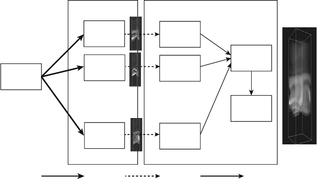
FIGURE 3.4: Visapult’s remote and distributed visualization architecture.
Image courtesy of E. Wes Bethel (LBNL).
3.8.1 Visapult Architecture: The Send-Geometry Partition
The original Visapult architecture, described by Bethel et al. 2000 [4],
shown in Figure 3.4, consists of two primary components. One component
is a parallel back end, responsible for loading scientific data and performing,
among other activities, “partial” volume rendering of the data set. The volume
rendering consists of applying a user-defined transfer function to the scalar
data, producing an RGBα volume, then performing axis-aligned compositing
of these volume subsets, producing semi-transparent textures. In a typical
configuration, each data block in the domain decomposition will result in six
volume rendered textures: one texture for each of the six principal axis viewing
directions. As a result, if the Visapult back end loads O(n
3
) data, it produces
O(n
2
) output in the form of textures.
Then, the back end transmits these “partially rendered” volume subsets
to the viewer, shown in Figure 3.4 as Partially Rendered Payload,where
the subsets are stored as textures in a high performance scene graph system
in the viewer. The viewer, via the scene graph system, renders these semi-
transparent textures on top of proxy geometry in the correct back-to-front
order at interactive rates via hardware-acceleration. Inside the viewer, the
scene graph system switches between each of the six source textures for each
data block depending upon camera orientation to present the viewer with the
best fidelity rendering.
38 High Performance Visualization
This particular “co-rendering” idea—where the server performs partial
rendering and the viewer finishes the rendering—was not new to Visapult.
Visapult’s architecture was targeted at creating a high performance, remote
and distributed visualization implementation of an idea called image-based
rendering assisted volume rendering described by Mueller et al. 1999 [20].
3.8.2 Visapult Architecture: The Send-Data Partition
Like all visualization applications, Visapult needs a source of data from
which to create images. Whereas modern, production-quality visualization
applications provide robust support for loading a number of well-defined file
formats, Visapult’s data source for all SC Bandwidth Challenge runs were
remotely located network data caches as opposed to files.
In the SC 2000 implementation, source data consisted of output from a
combustion modeling simulation. The data was stored on a Distributed Paral-
lel Storage System (DPSS), which can be thought of as a high-speed, parallel
remote block-oriented data cache [30]. In this implementation, the Visapult
back end invoked DPSS routines, similar in concept to POSIX fread calls
that, in turn, loaded blocks of raw scientific data in parallel, from a remote
source and relied on the underlying infrastructure, the DPSS client library, to
efficiently move data over the network.
In an effort to make an even better use of the underlying network, Shalf
and Bethel, 2003 [27], extended Visapult to make use of a UDP-based “con-
nectionless” protocol. They connected to a freely-running simulation, which
provided a data source. This change resulted in the ability for the Visapult
back end to achieve unprecedented levels of network utilization, close to 100%
of the theoretical line rate, for sustained periods of time.
The TCP-based approach can be thought of as a process of “load a
timestep’s worth of data, then render it.” Additionally, because the under-
lying protocol is TCP-based, there was no data loss between remote source
and the Visapult back end.
Going to the UDP-based model required rethinking both the network pro-
tocol and the Visapult back end architecture. In the TCP approach, the Visa-
pult back end “requests” data, which is a “pull” model. In the UDP approach,
though, the data source streams out data packets as quickly as possible, and
the Visapult back end must receive and process these data packets as quickly
as possible. This approach is a “push” model. There is no notion of timestep
or frame boundary in this push model; the Visapult back end has no way of
knowing when all the data packets, for a particular timestep, are in memory.
After all, some of the packets may be lost as UDP does not guarantee packet
delivery. See Bethel and Shalf, 2005, [3] for more design change details and
see Shalf and Bethel, 2003, [27] for the UDP packet payload design.

Remote and Distributed Visualization Architectures 39
!
"
#
$#
%&$'
(&&
)
*+
,
---
#
#!
!
FIGURE 3.5: CRRS system components for a two-tile DMX display wall con-
figuration. Lines indicate primary direction of data flow. System components
outlined with a thick line are new elements from this work to implement
CRRS; other components outlined with a thin line existed in one form or
another prior to the CRRS work. Image source: Paul et al. 2008 [23].
3.9 Case Study: Chromium Renderserver
Paul et al. 2008 [23] describe Chromium Renderserver (CRRS), which is a
software infrastructure that provides the ability for one or more users to run
and view image output from unmodified, interactive OpenGL and X11 appli-
cations on a remote, parallel computational platform, equipped with graphics
hardware-accelerators, via industry-standard Layer 7 network protocols and
client viewers.
Like Visapult, CRRS has a multi-stage pipeline partitioning that uses both
send-geometry and send-images approaches. Figure 3.5 shows a high-level ar-
chitectural diagram of a two-node CRRS system. A fully operational CRRS
system consists of six different software components, which are built around
VNC’s remote framebuffer (RFB) protocol. The RFB protocol is a Layer 7
network protocol, where image data and various types of control commands
are encoded and transmitted over a TCP connection, between producer and
consumer processing components. The motivation for using RFB is because
it is well understood, and there exist (VNC) viewers for nearly all the cur-
rent platforms. One of the CRRS design goals is to allow an unmodified VNC
viewer application to be used as the display client in a CRRS application.
The CRRS general components are:
• The application is any graphics or visualization program that uses
OpenGL and/or Xlib for rendering. Applications need no modifications
to run on CRRS, but they must link with the Chromium faker library
..................Content has been hidden....................
You can't read the all page of ebook, please click here login for view all page.