
76 High Performance Visualization
the incoming portion of the image with the same part of the image that it
already owns. By continually swapping, all processes remain busy throughout
all rounds. In each round, neighbors are chosen twice as far apart, and image
portions exchanged are half as large as in the previous round. This is why
binary-swap is also called a distance-doubling and vector-halving communica-
tion algorithm in some contexts.
Since the mid-1990s when direct-send and binary-swap were first pub-
lished, numerous variations and optimizations to the basic algorithms have
appeared. The basic ideas are to reduce active image regions using the spa-
tial locality and sparseness present in many scientific visualization images, to
better load balance after such reduction, and to keep network and computing
resources appropriately loaded through scheduling. Some examples of each of
these ideas are highlighted below.
Run-length encoding images achieves lossless compression [1], and using
bounding boxes to identify the nonzero pixels is another way to reduce the
active image size [15]. These optimizations can minimize both communication
and computation costs.
Load balancing via scan line interleaving [29] assigns individual scan lines
to processes so that each process is assigned numerous disconnected scan lines
from the entire image space. In this way, active pixels are distributed more
evenly among processes, and workload is better balanced. The drawback is
that the resulting image must be rearranged once it is composited, which can
be expensive for large images.
The SLIC [28] algorithm combines direct-send with active-pixel encod-
ing, scan-line interleaving, and scheduling of operations. Spans of compositing
tasks are assigned to processes in an interleaved fashion. Another way to sched-
ule processes is to assign them different tasks. This is the approach taken by
Ramakrishnan et al. [26], who scheduled some processes to perform rendering
while others were assigned to compositing. The authors presented an optimal
linear-time algorithm to compute this schedule.
Image compositing has also been combined with parallel rendering for
tiled displays. The IceT library, (see Chap. 17) from Moreland et al. [19],
performs sort-last rendering on a per-tile basis. Within each display tile, the
processors that contributed image content to that tile perform either direct-
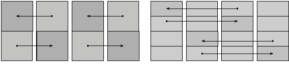
FIGURE 5.4: Example of the binary-swap algorithm for four processes and
two rounds.
Parallel Image Compositing Methods 77
send or binary-swap compositing. Although the tile feature of IceT is not used
much in practice, IceT has become a production-quality library that offers a
robust suite of image compositing algorithms to scientific visualization tools.
Both ParaView (see Chap. 18 and [32]) and VisIt (see Chap. 16 and [9]) use
the IceT library for image compositing.
5.2.3 Image Compositing Hardware
While this chapter primarily studies the evolution of software compositing
algorithms, it is worth noting that hardware solutions to the image com-
positing problem exist as well. Some of these have been made commercially
available on smaller clusters, but as the interconnects and graphics hardware
on visualization and HPC machines have improved over time, it has become
more cost-effective to use these general-purpose machines for parallel render-
ing and image compositing rather than purchasing dedicated hardware for
these tasks.
Sepia [16] is one example of a parallel rendering system that included PCI-
connected FPGA boards for image composition and display. Lightning-2 [27]
is a hardware system that received images from the DVI outputs of graphics
cards, composited the images, and mapped them to sections of a large tiled
display. Muraki et al. [20] described an eight-node Linux cluster equipped with
dedicated volume rendering and image composition hardware. In a more recent
system, the availability of programmable network processing units accelerated
image compositing across 512 rendering nodes [24].
5.3 Recent Advances
Although the classic image composition algorithms and optimizations have
been used for the past fifteen years, new processor and interconnect advances
such as direct memory access and multi-dimensional network topology present
new opportunities to improve the state of the art in image compositing. The
next few sections explain the relationship between direct-send and binary-
swap through a tree-based representation and how it is used to develop more
general algorithms that combine both techniques. Two recent algorithms, 2-3
swap and radix-k, are presented as examples of more general communication
patterns that can exploit new hardware.
5.3.1 2-3 Swap
Yu et al. [33] extended binary-swap compositing to nonpower-of-two num-
bers of processors with an algorithm they called 2-3 swap. One goal of this
algorithm is to combine the flexibility of direct-send with the scalability of
binary-swap, and the authors accomplished this by recognizing that direct-
send and binary-swap are related and can be combined into a single algorithm.

78 High Performance Visualization
FIGURE 5.5: Example of the 2-3 swap algorithm for seven processes in two
rounds. Group size is two or three in the first round, and between two and
five in the second round.
Any natural number greater than one can be expressed as the sum of
twos and threes, and this property is used to construct the first-round group
assignment in the 2-3 swap algorithm. The algorithm proceeds to execute a
sequence of rounds with group sizes that are between two and five. Each round
can have multiple group sizes present within the same round. The number of
rounds, r, is equal to the base of log p,wherep is the number of processes and
need not be a power of two, as is the case for the binary-swap algorithm.
An example of 2-3 swap using seven processes is shown in Figure 5.5. In
the first round, shown on the left, processes form groups in either twos or
threes, as the name 2-3 swap suggests, and execute a direct-send within each
group. (Direct-send is the same as binary-swap when the group size is two.)
In the second round, shown on the right, the image pieces are simply divided
into a direct-send assignment, with each process owning 1/p,or1/7inthis
example, of the image. By assigning which 1/7 each process owns, however,
Yu et al. proved that the maximum number of processes in a group is five,
avoiding the contention in the ordinary direct-send. Indeed, Figure 5.5 shows
that process P
5
receives messages from four other processes, while all other
processes receive messages from only two or three other processes.
5.3.2 Radix-k
The next logical step in combining and generalizing direct-send and binary-
swap is to allow more combinations of rounds and group sizes. To see how
this is done, let k
i
represent the number of processes in a communication

Parallel Image Compositing Methods 79
FIGURE 5.6: Example of the radix-k algorithm for twelve processes, factored
into two rounds of
k =[4, 3].
group in round i. The k-values for all rounds can be written as the vector
k =[k
1
,k
2
, ..., k
r
], where the number of rounds is denoted by r. Within each
group, a direct-send is performed. The total number of processes is p.
More than a convenient notation, this terminology makes clear the rela-
tionship among the previous algorithms. Direct-send is now defined as r =1
and
k =[p]; and binary-swap is defined as r =logp and
k =[2, 2, 2, ...]. Just
as 2-3 swap was an incremental step in combining direct-send and binary-swap
by allowing k-values that are either 2 or 3, it is natural to ask whether other
combinations of r and
k are possible. The radix-k algorithm [22] answers this
question by allowing any factorization of p into
r
i=1
k
i
= p. In radix-k, all
groups in round i are the same size, k
i
.
Figure 5.6 shows an example of radix-k for p =12and
k =[4, 3]. The
processes are drawn in a 4 × 3 rectangular layout to identify the rounds and
groups clearly. In this example, the rows on the left side form groups in the
first round, while the columns on the right side form second-round groups. A
convenient way to think about forming groups in each round is to envision
the process space as an r-dimensional virtual lattice, where the size in each
dimension is the k-value for that round. This is the convention followed in
Figure 5.6 for two rounds drawn in two dimensions.
The outermost rectangles in the figure represent the image held by each
process at the start of the algorithm. During the round i, the current image
piece is further divided into k
i
pieces, such that the image pieces grow smaller
with each round. The image pieces are shown as highlighted boxes in each
round.
Selecting different parameters can lead to many options; for the example
80 High Performance Visualization
above, other possible parameters for
k are [12], [6, 2], [2, 6], [3, 4], or [2, 2, 3],
to name a few. With a judicious selection of
k, higher compositing rates are
attained when the underlying hardware offers support for multiple commu-
nication links and the ability to perform communication and computation
simultaneously. Even when hardware support for increased parallelism is not
available or the image size or number of processes dictates that binary-swap
or direct-send is the best approach, those algorithms are valid radix-k config-
urations.
5.3.3 Optimizations
Kendall et al. [11] extended radix-k to include active-pixel encoding and
compression, and they showed that such optimizations benefit radix-k more
than its predecessors, because the choice of k-values is configurable. Hence,
when message size is decreased by active-pixel identification and encoding,
k-values can be increased and performance can be further enhanced. Their
implementation encodes nonempty pixel regions, based on the bounding box
information, into two separate buffers: one for alternating counts of empty
and nonempty pixels, and the other for the actual pixel values. This way,
new subsets of the image can be taken by reassigning pointers rather than
copying pixels, and images remain encoded throughout all of the composit-
ing rounds. Non-overlapping regions are copied from one round to the next
without performing the blending operation.
A set of empirical tests was performed to determine a table of target k-
values for different image sizes, number of processes, and architectures at both
the Argonne and Oak Ridge Leadership Computing Facilities. The platforms
tested were IBM Blue Gene/P, Cray XT, and two graphics clusters. With this
table, radix-k can look up the closest entry for a given image size, system
size, and architecture, and automatically factor the number of processes into
k-values as close to the target value as possible.
Moreland et al. [18] deployed and evaluated optimizations in a production
framework, rather than in isolated tests: IceT serves as both this test and
production framework. The advantages of this approach are that the tests
represent real workloads and improvements are ready for use in a production
environment sooner. These improvements include minimizing pixel copying
through compositing order and scanline interleaving, and a new telescoping
algorithm for the non-power-of-two number of processes that can further im-
prove radix-k. A final advantage of using IceT for these improvements is that
IceT provides unified and reproducible benchmarks that other researchers can
repeat.
One of the improvements was devising a compositing order that minimizes
pixel copying. The usual, accumulative order causes nonoverlapping pixels to
be copied up to k
i
−1 times in round i, whereas tree methods only incur log k
i
copy operations. Pixel copying can further be reduced while using a novel
image interlacing algorithm. Rather than interleaving partitions according to
..................Content has been hidden....................
You can't read the all page of ebook, please click here login for view all page.