

Parallel Integral Curves 101
of slave processes. Each master is responsible for monitoring the workload
among the group of slaves, and making work assignments that optimize re-
source utilization. The master makes initial assignments to the slaves based on
the initial seed point placement. As work progresses, the master monitors the
length of each slave’s work queue and the blocks that are loaded. The master
reassigns particle computation to balance both slave overload and slave star-
vation. When the master determines that all streamlines have terminated, it
instructs all slaves to terminate.
For scalable performance, work groups coordinate between themselves and
work can be moved from one work group to another, as needed. This allows
for work groups to focus resources on different portions of the problem, as
needed.
The design of the slave process is outlined in Algorithm 3. Each slave
continuously advances particles that reside in data blocks that are loaded.
Similarly, to the parallelize over seed points algorithm, the data blocks are
held in an LRU cache to the extent permitted by the memory. When the slave
cannot advance any more particles or is out of work, it sends a status message
to the master and waits for further instruction. In order to hide latency, the
slave sends the status message right before it advances to the last particle.
Algorithm 3 Slave Process Algorithm
while not done do
if new command from master then
process command
end if
while active particles do
process particles
end while
if state changed then
send state to master
end if
end while
The master process is significantly more complex, and outlined at a high
level in Algorithm 4. The master process is responsible for maintaining infor-
mation on each slave and managing their workloads. At regular intervals, each
slave sends a status message to the master so that it maintains accurate global
information. This status message includes: the set of particles owned by each
slave, which data blocks those particles currently intersect, which data blocks
are currently loaded into memory on that slave, and how many particles are
currently being processed. The master enforces load balancing by monitor-
ing the workload of the group of slaves, and deciding dynamically, how work
should be shared. This is done using particle reassignment, and redundantly
loading data blocks. All communication is performed using non-blocking send
and receive commands.

102 High Performance Visualization
Algorithm 4 Master Process Algorithm
get initial particles
while not done do
if New status from any slave then
command ← most efficient next action
Send command to appropriate slave(s)
end if
if New status from another master then
command ← most efficient next action
Send command to appropriate slave(s)
end if
if Work group status changed then
Send status to other master processes
end if
if All work groups done then
done = true
end if
end while
The master process uses a set of four rules to manage the work in each
group. The rules are:
1. Assign loaded block. The master sends a particle to a slave that has the
required data block already loaded into memory. The slave will add this
particle to the active particle list and process the particle.
2. Assign unloaded block. The master sends a particle to a slave that does
not have the required data block loaded into memory. The slave will
load the data block into memory, add the particle to its active particle
list, and process the particle. The master process uses this rule to assign
the initial work to slaves when particle advection begins.
3. Load block. The master sends a message to a slave instructing it to load
a data block required by one or more of the assigned particles. When the
slave receives this message, the data block is loaded, and the particles
requiring this data block are moved into the active particle list.
4. Send particle. The master sends a message to a slave instructing it to
send particles to another slave. When the slave receives this command,
the particle is sent to the receiving slave. The receiving slave will then
place this particle in the active particle list.
The master in each work group monitors the load of the set of slaves.
Using a set of heuristics [11], the master will use the four commands above
to dynamically balance work across the set of slaves. The commands allow
particle, and data block assignments for each processor to be changed over
the course of the integration calculation.
Parallel Integral Curves 103
6.3.5 Algorithm Analysis
The efficiency of the three algorithms are compared by applying each algo-
rithm to several representative data sets and seed point distribution scenarios
and by measuring various aspects of performance. Because each algorithm
parallelizes differently over the particles and blocks, it is insightful to ana-
lyze the performance of the total runtime and also other key metrics that are
impacted directly by the parallelization strategy choices.
One overall metric of the analysis is the total runtime or wall-clock time
of the algorithm. This metric includes the total time-to-solution of each al-
gorithm, including IC computation, I/O, and communication. Although, this
metric alone is not sufficiently fine-grained enough to capture or convey per-
formance characteristics of an algorithm on a given data set with a given
initial seed set. The analysis of communication, I/O, and block management
gives a more fine-grained insight into the performance efficiency.
Communication is a difficult metric to report and analyze since all commu-
nication in these algorithms are asynchronous. However, the time required to
post send and receive operations and associated communication management
measures the impact of parallelization that involves communication.
To measure the impact of I/O upon parallelization, time spent reading
blocks from a disk is recorded, as well as the number of times blocks are loaded
and purged. Because not all the blocks will fit into memory, an LRU cache,
with a user-defined upper bound, is implemented to handle block purging. A
ratio measures the efficiency of this aspect of the algorithm, which is defined
by the block efficiency, E. The block’s efficiency is the difference between
number of blocks loaded and the number of blocks purged, over the number
of blocks loaded.
E =
B
L
− B
P
B
L
. (6.1)
For the astrophysics data set, the wall-time graph in Figure 6.5a demon-
strates the relative time performance of the three algorithms, with the hybrid
parallelization algorithm demonstrating a better performance than either seed
parallelization or data parallelization, for both spatially sparse and dense ini-
tial seed points. However, even at 512 processors, the difference between hybrid
and data parallelization for the spatially sparse seed point set is only a factor
of 3.8, so, in order to understand the parallelization, the analysis must include
other metrics.
An examination of total time spent in I/O, as shown in Figure 6.5b, is
particularly informative. In this graph, the hybrid algorithm performs very
close to the ideal, as exemplified by the data parallelization algorithm. Though
seed parallelization performs closely to the hybrid approach from a time point
of view, it spends an order of magnitude more time in I/O for both seed point
initial conditions.
Next, the block efficiency (see Eq. 6.1), is shown in Figure 6.5c for all three
algorithms. The data parallelization performs ideally, loading each block once

104 High Performance Visualization
FIGURE 6.5: Graphs showing performance metrics for parallelization over
seeds, parallelization over data and hybrid parallelization algorithms on the
astrophysics data set. There were 20,000 particles used with both sparse and
dense seeding scenarios. Image source: Pugmire et al., 2009 [11].
and never purging. The seed parallelization performs least efficiently, as blocks
are loaded and reloaded many times. The performance of the hybrid algorithm
is close to ideal for both sparse and dense seeding, which highlights the ability
to dynamically direct computational resources, as needed.
It is also useful to consider the time spent in communication, shown in
Figure 6.5d. As the seed parallelization algorithm does no communication,
times are only shown for data and hybrid parallelization. For sparse seeding,
data parallelization performs approximately 20 times more communication
than the hybrid algorithm as ICs are sent between the processors that own
the blocks. This trend remains even as the number of processors is scaled up.
For the dense initial condition, the separation increases by another order of
magnitude, as data parallelization performs between 165 and 340 times more
communication as the processor count increases. This is because the ratio of
blocks needed to total blocks decreases and large numbers of ICs communicate
to the processors that own the blocks.
For the fusion data set, the wall-time graph in Figure 6.6a demonstrates
the relative time performance of the three algorithms. In the fusion data set,
the nature of the vector field, which rotates within the toroidal containment
core, leads to some interesting performance results. Because of this, regardless
of seed placement, the ICs tend to uniformly fill the interior of the torus.
The data parallelization and hybrid algorithms perform almost identically for
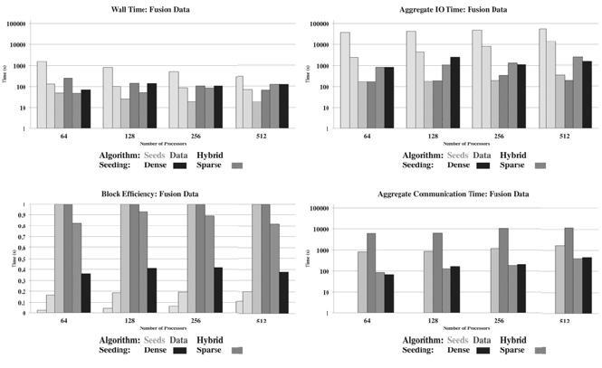
Parallel Integral Curves 105
FIGURE 6.6: Graphs showing performance metrics for parallelization over
seeds, parallelization over data and hybrid algorithms on the fusion data set.
There were 20,000 particles used with both sparse and dense seeding scenarios.
Image source: Pugmire et al., 2009 [11].
both seeding conditions. The seed parallelization algorithm performs poorly
for spatially sparse seed points, but very competitively for a dense seed points.
In the case of seed parallelization with a dense seeding, good performance
is obtained because the working set of active blocks fits inside memory and
few blocks must be purged to advance the ICs around the toroidal core. An
analysis of wall-clock time does not clearly indicate a dominant algorithm be-
tween data and hybrid parallelization, so further analysis is warranted. But it
is encouraging that the hybrid algorithm can adapt to both initial conditions.
The graph of total I/O time is shown in Figure 6.6b. In both seeding sce-
narios, as expected, seed parallelization performs more I/O; however, it does
not have the communication costs and latency of the other two algorithms and
so, for the case of the dense seeding, seed parallelization is able to overcome
the I/O penalty to show good performance overall.
The graph of block efficiency is shown in Figure 6.6c. It is interesting
to note that the block efficiency of the hybrid algorithm is less than in the
astrophysics case study. However, overall performance is still very strong. This
indicates that for this particular data set, the best overall performance is found
when more blocks are replicated across the set of resources.
The graph of total communication time is shown in Figure 6.6c. For a dense
seeding, communication is very high for the data parallelization algorithm.
Since the ICs tend to be concentrated in an isolated region of the torus,
..................Content has been hidden....................
You can't read the all page of ebook, please click here login for view all page.