
106 High Performance Visualization
many ICs must be communicated to the block owning processors. For sparse
seeding, the ICs are more uniformly distributed and communication costs are
therefore lower.
6.3.6 Hybrid Data Structure and Communication Algorithm
Large seed sets and large time-varying vector fields pose additional chal-
lenges for parallel IC algorithms. The first challenge is the decomposition
of 4D time-varying flow data, in space and time. This section discusses a
hybrid data structure that combines both 3D and 4D blocks for comput-
ing time-varying ICs efficiently. The second challenge arises in both steady
and transient flows but it is magnified in the latter case: this is the problem
of performing nearest-neighbor communication iteratively while minimizing
synchronization points during the execution. A communication algorithm is
introduced, then, for the exchange of information among neighboring blocks
that allows tuning the amount of synchronization desired. Together, these
techniques are used to compute 1/4 million steady-state and time-varying
ICs on vector fields over 1/2 terabyte in size [10].
Peterka et al. [9] introduced a novel 3D/4D hybrid data structure, which is
shown in Figure 6.7. It is called “hybrid” because it allows a 4D space–time to
be viewed as both a unified 4D structure and a 3D space × 1D time structure.
The top row of Figure 6.7 illustrates this idea for individual blocks, and the
bottom row shows the same idea for neighborhoods of blocks.
The same data structure is used for both steady-state and time-varying
flows, by considering steady-state as a single timestep of the time-varying gen-
eral case. After all, a particle is a 4D (x, y, z, t) entity. In the left column of
Figure 6.7, a block is also a 4D entity, with both minimum and maximum
extents in all four dimensions. Each 4D block sits in the center of a 4D neigh-
borhood, surrounded on all sides and corners by other 4D blocks. A single
neighborhood consists of 3
4
blocks: the central block and adjacent blocks are
in both directions in the x, y, z,andt dimensions.
If the data structure were strictly 4D, and not hybrid, the center and right
columns of Figure 6.7 would be unnecessary; but then, all timesteps of a time-
varying flow field would be needed at the same time, in order to compute an
IC. Modern CFD simulations can produce hundreds or even thousands of
timesteps, and the requirement to simultaneously load the entire 4D data set
into a main memory would exceed the memory capacity of even the largest
HPC systems. At any given time in the particle advection, however, it is only
necessary to load data blocks that contain vector fields at the current time
and perhaps one timestep in the future. On the other hand, loading multiple
timesteps simultaneously often results in a more efficient data access pattern
from storage systems and reduced I/O time. Thus, the ability to step through
time in configurable-sized chunks, or time windows, results in a flexible and
robust algorithm that can run on various architectures with different memory
capacities.

Parallel Integral Curves 107
FIGURE 6.7: The data structure is a hybrid of 3D and 4D time–space de-
composition. Blocks and neighborhoods of blocks are actually 4D objects. At
times, such as when iterating over a sliding time window (or time block) con-
sisting of one or more timesteps, it is more convenient to separate 4D into 3D
space and 1D time. Image courtesy of Tom Peterka (ANL).
Even though blocks and neighborhoods are internally unified in space–
time, the hybrid data structure enables the user to decompose space–time
into the product of space × time. The lower right corner of Figure 6.7 shows
the decomposition for a temporal block consisting of a number of individual
timesteps. Varying the size of a temporal block—the number of timesteps
contained in it—creates an adjustable sliding time window that is also a con-
venient way to trade the amount of in-core parallelism with out-of-core seri-
alization. Algorithm 5 shows this idea in pseudocode. A decomposition of the
domain into 4D blocks is computed given user-provided parameters, specify-
ing the number of blocks in each dimension. The outermost loop then iterates
over 1D temporal blocks, while the work in the inner loop is done in the con-
text of 4D spatio-temporal blocks. The hybrid data structure just described,
enables this type of combined in-core/out-of-core execution, and the ability to
configure block sizes in all four dimensions is how Algorithm 5 can be flexibly
tuned to various problem and machine sizes.
All parallel IC algorithms for large data and seed sets have one thing in
common: the inevitability of interprocess communication. Whether exchang-
ing data blocks or particles, nearest-neighbor communication is unavoidable
and limits performance and scalability. Hence, developing an efficient nearest-
neighbor communication algorithm is crucial. The difficulty of this communi-
cation stems from the fact that neighborhoods, or groups in which communi-
cation occurs, overlap. In other words, blocks are members of more than one

108 High Performance Visualization
Algorithm 5 Main Loop
decompose entire domain into 4D blocks
for all 1D temporal blocks assigned to my process do
read corresponding 4D spatio-temporal data blocks into memory
for all 4D spatio-temporal blocks assigned to my process do
advect particles
end for
end for
neighborhood: a block at the edge of one neighborhood is also at the center
of another, and so forth. Hence, a delay in one neighborhood will propagate
to another, and so on, until it affects the entire system. Reducing the amount
of synchronous communication can absorb some of these delays and improve
overall performance and one way to relax such timing requirements is to use
nonblocking message passing.
In message-passing systems like MPI, nonblocking communication can be
confusing. Users often have the misconception that communication automat-
ically happens in the background, but in fact, messages are not guaranteed
to make progress without periodic testing of their status. After nonblocking
communication is initiated, control flow is returned to the caller and hope-
fully, some communication occurs while the caller executes other code, but to
ensure this happens, the caller must periodically check on the communication
and perhaps wait for it to complete.
The question then becomes how frequently one should check back on non-
blocking messages, and how long to wait during each return visit. An efficient
communication algorithm that answers these questions was introduced by Pe-
terka et al. [10] and is outlined in Algorithm 6. The algorithm works under
the assumption that nearest-neighbor communication occurs in the context of
alternating rounds between the advection and communication of particles. In
each round, new communication is posted and previously posted messages are
Algorithm 6 Asynchronous Communication Algorithm
for all processes in my neighborhood do
pack message of block IDs and particle counts
post nonblocking send
pack message of particles
post nonblocking send
post nonblocking receive for IDs and counts
end for
wait for enough IDs and counts to arrive
for all IDs and counts that arrived do
post blocking receive for particles
end for

Parallel Integral Curves 109
FIGURE 6.8: The cumulative effect on end-to-end execution time of a hybrid
data structure and an adjustable communication algorithm is shown for a
benchmark test of tracing 256K particles in a vector field that is 2048 ×
2048 × 2048.
checked for progress. Each communication consists of two messages: a header
message containing block identification and particle counts, and a payload
message containing the actual particle positions.
The algorithm takes an input parameter that controls the fraction of pre-
viously posted messages for which to wait in each round. In this way, the
desiredamountofsynchrony/asynchronycanbeadjustedandallowsthe“di-
aling down” of synchronization to the minimum needed to make progress. In
practice, waiting for only 10% of the pending messages to arrive in each round
is the best setting. This way, each iteration makes a guaranteed minimum
amount of communication progress, without imposing excessive synchroniza-
tion. Reducing communication synchronization accelerates the overall parti-
cle advection performance and is an important technique for communicating
across large-scale machines where global code synchronization becomes more
costly as the number of processes increases.
The collective effect of these improvements is a 2× speedup in overall
execution time, compared to earlier algorithms. This improvement is demon-
strated in Figure 6.8 with a benchmark test of tracing 1/4 million particles in
a steady state thermal hydraulics flow field that is 2048
3
in size. Peterka et
al. [10] benchmarked this latest fully-optimized algorithm using scientific data
sets from problems in thermal hydraulics, hydrodynamics (Rayleigh–Taylor
instability), and combustion in a cross-flow. Table 6.1 shows the results on
110 High Performance Visualization
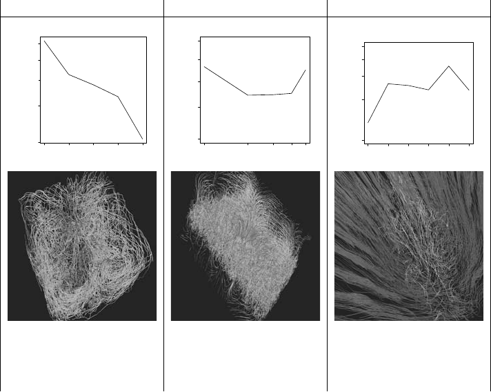
TABLE 6.1: Parallel IC performance benchmarks.
Thermal Hydraulics Hydrodynamics Combustion
100 150 200 250 300
Strong Scaling
Number of Processes
Time (s)
1024 2048 4096 8192 16384
Strong Scaling
Number of Processes
100
150
200
Time (s)
250
300
1024 2048 4096 8192 16384
200 250 300 350 400
Weak Scaling by Increasing No. of Particles
Number of Processes
Time (s)
4096 8192 12288 16384 20480
Weak Scaling by Increasing No. of Particles
Number of Processes
Time (s)
200 250 300 350 400
4096 8192 12288 16384 20480
100 200 300 400 500
Weak Scaling by Inreasing No. of Particle and Time Steps
Number of Processes
Time (s)
128 256 512 1024 2048 4096
100
Time (s)
Weak Scaling by Increasing No. of
Particles and Time Steps
128 256 512 1024 2048
Number of Processes
4096
200 300 400 500
Strong scaling, 2048
× 2048 × 2048 × 1
timestep = 98GB data,
128K particles
Weak scaling, 2304
× 4096 × 4096 × 1
timestep = 432GB data,
16K to 128K particles
Weak scaling, 1408
× 1080 × 1100 × 32
timesteps = 608GB data,
512 to 16K particles
both strong and weak scaling tests of steady and unsteady flow fields. The
left-hand column of Table 6.1 shows good strong scaling (where the problem
size remains constant) for the steady-state case, seen by the steep downward
slope of the scaling curve. The center column of Table 6.1 also shows good
weak scaling (where the problem size increases with process count), with a flat
overall shape of the curve. The right-hand column of Table 6.1 shows a weak
scaling curve that slopes upward for the time-varying case and it demonstrates
that even after optimizing the communication, the I/O time to read each time
block from storage remains a bottleneck.
Advances in hybrid data structures and efficient communication algorithms
can enable scientists to trace particles of time-varying flows during their sim-
ulations of CFD vector fields at a concurrency that is comparable with their
parallel computations. Such highly parallel algorithms are particularly impor-
tant for peta- and exascale computing, where more analyses will be needed
to execute at simulation runtime, in order to avoid data movement and avail
full-resolution data at every time step. Access to high-frequency data that are
only available in situ is necessary for accurate IC computation; typically, sim-
..................Content has been hidden....................
You can't read the all page of ebook, please click here login for view all page.