

150 High Performance Visualization
Each set S
j
is a subset of S
j+1
. To avoid data replication a set differences is
constructed, such that:
S
j
= S
j
− S
j−1
.
S
j
is then stored, instead of S
j
. Reconstructing S
j
from S
j
requires reading
all S
i
,where0≤ i ≤ j, and forming the union S
j
= S
0
∪ ...∪ S
j
.Ineachof
the Figures 8.1a–d, a circle enclosed inside a square is used to denote a grid
point added through the union of the sets S
j
and S
j−1
.
There are a few additional properties of the Z-order curve that are helpful
to support the construction and access of S
j
.
The level in the hierarchy that a point with Z-order curve index z belongs
to is given by:
j =
0ifz =0,
j
max
−
n
d
if z>0,
(8.1)
where 2
n
is the largest power-of-two factor of z.
The cardinality of S
j
is
|S
j
| =
1ifj =0,
2
dj
− 2
d(j−1)
if j>0.
(8.2)
Finally, the z value from a point in the set S
j
can be reconstructed as:
z =(l +
l
2
d
− 1
+1)2
d(j
max
−j)
, (8.3)
where l is the integer offset of the point within the set (recall set elements are
ordered by z).
When reordering data on disk from row (column) major order to Z-order
curve, Equation 8.1 allows the user to walk the Z-order curve and determine
what point belongs to which set of S
j
. When reconstructing row (column)
major order from Z-order curve data stored on disk, Equation 8.3 provides a
point’s z offset based on its position in S
j
.
There are a few other items worth noting. No floating point calculations
are performed on the data in the scheme described above and the storage of
the data is simply reordered in a manner that lends itself to progressive access
and subregion extraction. Hence, the reconstructed data at the highest level of
the hierarchy are bit-for-bit identical to the original data. In general, this will
not be true of other progressive access models. A less desirable aspect of the
approach is that data coarsening is performed through simple subsampling.
The quality of the coarsened approximations will not be as high as when
achieved by other methods.

Progressive Data Access for Regular Grids 151
8.4 Wavelets
In the preceding section, the Z-order curve offers a convenient way to create
and access a multiresolution hierarchy composed of the nodes of a gridded
hypercube. While the method allows for bit-for-bit identical reconstruction of
the original grid and does not impose any additional storage overhead, the
restriction to the grids with regular symmetry and power-of-two dimensions,
or the crudeness of coarsened approximations created by sub-sampling, may
prove limiting. In this section, both of these shortcomings are addressed, but
they give up exact, bit-for-bit reconstruction.
Consider the following set of samples from a 1D signal:
c
3
[n]=[13359775].
The eight samples can be approximated with pair-wise, unweighted averaging
to produce signal at half the resolution:
c
2
[
n
2
]=[2486].
The samples in c
2
[
n
2
] are constructed by
c
j−1
[i]=
1
2
(c
j
[2i +1]+c
j
[2i]). (8.4)
Now consider the signal constructed with
d
j−1
[i]=
1
2
(c
j
[2i +1]− c
j
[2i]). (8.5)
So, for the d
2
[
n
2
] example:
d
2
[
n
2
]=[11−1 −1].
The signal d
2
[
n
2
], when combined with c
2
[
n
2
], provides a way to reconstruct
the original c
3
[n]:
c
j
[2i]=c
j−1
[i] − d
j−1
[i],
c
j
[2i +1]=c
j−1
[i]+d
j−1
[i].
(8.6)
The samples in c
j
are referred to as approximation coefficients, and those
in d
j
, which represent the differences or the error introduced by averaging two
neighboring data values, are referred to as detail coefficients. The calculations
given by Equations 8.4 and 8.5 can be recursively applied to c
j
until a single
approximation coefficient is left—the average of all the samples in our original
signal—and, in this example, seven detail coefficients:
c
0
,d
0...2
=[521−111−1 −1].
Thus, a linear transform has been applied to the original signal that allows
152 High Performance Visualization
0
2
00
4
00 600 800
1
000
−80
−60
−40
−20
0
20
40
60
(a)
0
2
0
4
0 60 80
1
00
12
0
−80
−60
−40
−20
0
20
40
60
(b)
0
2
0
4
0 60 80
1
00
12
0
−80
−60
−40
−20
0
20
40
60
(c)
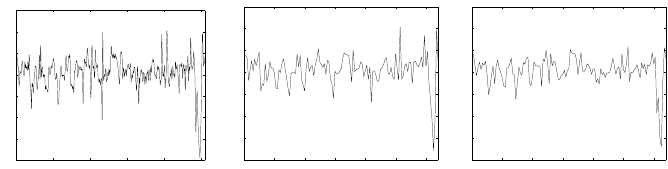
FIGURE 8.2: PDA based on multiresolution. The original signal containing
1024 samples (a), reduced to 1/8
th
resolution using subsampling, analogous
to the Z-order curve (b); and the Haar wavelet approximation coefficients (c).
a reconstruction of an approximation with 1, 2, 4, or 8 samples, but with-
out any storage overhead. In the context of data read from disk, the coarsest
approximation, c
0
, can be retrieved by reading a single sample, the next ap-
proximation level, c
1
, by reading one additional coefficient, d
0
, and applying
Equation 8.6, and the next, by reading two more coefficients, and so on. Multi-
ple dimensions can be easily generalized by averaging neighboring points along
each dimension to generate approximation coefficients, and generate detail co-
efficients by taking the difference between the approximation coefficients and
each of the points used to find its average.
Mathematically, this is the 1D, unnormalized, Haar wavelet transform.
The Haar wavelet transform, and other wavelet transforms that are discussed
later, constructs a multiresolution representation of a signal. In one dimension,
each multiresolution level j contains, on average, half the samples of the j +1
level approximation, with coarser level samples created by averaging finer
level samples. Note, while the Haar transform exhibits what is known in the
digital signal processing world as the property of perfect reconstruction, due
to limited floating point precision the signal reconstructed from the c
j
and
d
j
coefficients will not, as was the case with the Z-order curve, be an exact
copy of the original signal. Moreover, even if the input signal consists entirely
of the integer data the division by two in Equation 8.4 will result in floating
point coefficients. However, integer-to-integer wavelet transforms do exist [3],
but they are not discussed here.
Figure 8.2 shows a qualitative comparison of a 1D sampling of the x-
component of vorticity obtained from a 1024
3
simulation by Taylor-Green
turbulence [7]. The original signal is seen in Figure 8.2a. The signal generated
by nearest neighbor sampling (analogous to Z-order curve approximation) at
1/8
th
resolution is shown in Figure 8.2b, and at the same coarsened resolution,
approximated with the Haar wavelet, as in Figure 8.2c.
Equations 8.4–8.6 provide everything that is needed to support a PDA
scheme based purely on a multiresolution hierarchy, not suffering from the
Progressive Data Access for Regular Grids 153
limitations of the Z-order curve, but giving up bit-for-bit identical reconstruc-
tion. One drawback of both the Z-order curve and the wavelet based multires-
olution approach is that they fail to take advantage of any coherence in the
data. Better approximations of a function can be achieved for a given number
of coefficients, by further exploiting some of the properties of wavelets.
8.4.1 Linear Decomposition
Often it is advantageous to represent a signal or function f as a superpo-
sition:
f(t)=
k
a
k
u
k
(t) k ∈ Z,a∈ R, (8.7)
where a’s are expansion coefficients,andu
k
(t)’s are a set of functions of time,
t, that form a basis for L
2
—the space of square, integrable (finite energy) func-
tions. If, for example, u
k
’s are complex exponentials, then the expansion is a
Fourier series of f. More generally, if the basis functions, u
k
(t), are orthogonal,
that is if
u
k
(t),u
l
(t) =
u
k
(t)u
l
(t)dt =0 l = k (8.8)
then the coefficients a
k
can be easily calculated by the inner product:
a
k
= f (t),u
k
(t) =
f(t)u
k
(t)dt. (8.9)
The wavelet expansions of signals are also superpositions of basis functions
but they are represented as a two-parameter expression:
f(t)=
k
c
j
min
,k
φ
j
min
,k
(t)+
j
k
d
j,k
ψ
j,k
(t), (8.10)
where c
j,k
and d
j,k
are again real-value coefficients. φ
j,k
(t)andψ
j,k
(t)are
the scaling and wavelet basis functions, respectively. The parameterization of
time (or space) is provided by k, while frequency or scale, not coincidentally,
is parameterized by j.
Several properties of wavelets and the above wavelet expansion are appli-
cable to all wavelets discussed in this section:
1. The wavelet expansion computes efficiently. For discrete f(t), the upper
bound on the parameter j is log
2
(N), where N is the number of samples
in f . Similarly, for many wavelets both φ
j,k
(t)andψ
j,k
(t)havecompact
support and are zero-valued outside of a small interval of t.Thus,the
expansion is computed with only a handful of multiplications and ad-
ditions, making its complexity O(N ).Thesameistrueforthewavelet
transform used to compute c
j,k
and d
j,k
. Compare this to O(Nlog
2
(N))
complexity for the Fourier expansion.

154 High Performance Visualization
2. Unlike the Fourier transform, the wavelet transform localizes in time
(space) the frequency information of a signal. Most of the information
or energy of a signal is represented by a small number of expansion
coefficients (a property exploited later for progressive data access).
3. Finally, Equation 8.10 provides a multiresolution decomposition of f.
The first term of the right-hand side of the equation describes a coars-
ened, low-resolution approximation of f , while the second term, for in-
creasing j, provides finer and finer details—that represent the missing
information not contained in the first term. Another view is that the
first term contains the low frequency components of f, while the second
term provides the high frequency components of f. Hence, the labels
approximation and detail are applied to the coefficients, c
j
and d
j
,re-
spectively.
8.4.2 Scaling and Wavelet Functions
Up to this point, scaling and wavelet functions have been discussed with-
out formally defining them. Unlike the Fourier basis functions, the complex
exponentials, the wavelet and scaling functions are an infinitely large family of
functions. Here, the discussion will strictly pertain to normalized, orthogonal,
or orthonormal, families of wavelets as defined by the relations:
φ
j,k
(t),φ
j,l
(t) = δ(k, l)
ψ
j,k
(t),ψ
j,l
(t) = δ(k, l)
φ
j,k
(t),ψ
j,l
(t) =0
⎫
⎪
⎬
⎪
⎭
for all j, k, and l, (8.11)
where δ(k, l)is1fork = l, otherwise δ(k, l)is0.
The multiresolution properties of the wavelet expansion arise from the
scaling function and the ability to recursively construct this basis function
from a canonical version of itself. That is
φ(t)=
n
h
0
[k]
√
2φ(2t − n) n, k ∈ Z. (8.12)
Equation 8.12 is a dilation equation; it shows how to construct the scaling
function, φ(t), from the superposition of scaled, translated, and dilated copies
of itself. The translation (t − n) shifts φ(t) to the right. The multiplier 2t
narrows (dilates) φ(t), and
√
2 scales the function. In other words, φ(t)is
expressed as a linear expansion, similar in form to Equation 8.7, but by using
itself as a basis! By convention, the expansion coefficients are relabeled from
a
k
to h
0
[k].
For the Haar basis function discussed in the beginning of 8.4, the canonical
form of φ(t)is:
..................Content has been hidden....................
You can't read the all page of ebook, please click here login for view all page.