

Progressive Data Access for Regular Grids 155
φ(t)=
10≤ t<1,
0 otherwise.
(8.13)
Thus, the Haar scaling function is a box of unit height over the interval [0, 1).
The expansion coefficients, h
0
[k], for the Haar scaling function are h
0
[0] =
h
0
[1]=1/
√
2.
Using shifted, scaled, and dilated versions of the scaling function φ(t)alone,
we can construct a multiresolution hierarchy of f(t). However, much like the
first attempt with the Z-order curve, this leads to more replications. For these
and other reasons that are beyond the scope of this text, the wavelet expansion
includes a second basis function, ψ(t), that provides a means to capture the
information that is missing from the approximation based on φ(t).
Similar to the scaling functions, the wavelets are also defined by the canon-
ical scaling function:
ψ(t)=
n
h
1
[k]
√
2φ(2t − n). (8.14)
Here, h
1
are a different set of expansion coefficients from h
0
. Without proof,
the orthogonal wavelets h
0
and h
1
are related to each other by
h
1
[n]=(−1)
n
h
0
(N − 1 − n), (8.15)
where N is the support size of h
0
.
Thus, for the Haar wavelet, the non-zero coefficients in Equation 8.14 are
h
1
[0] = 1/
√
2andh
1
[1] = −1/
√
2. The canonical Haar wavelet function is
therefore:
ψ(t)=
⎧
⎪
⎨
⎪
⎩
10≤ t<1/2,
−11/2 ≤ t<1,
0 otherwise.
(8.16)
A multitude of wavelet families exist, each with a variety of parameteri-
zations. A reasonable question to ask is: If Haar wavelets possess all of the
multiresolution properties required, why consider other wavelets? Again, an
in-depth treatment is beyond the scope of this text, and the remarks will be
limited to those properties related only to the goals of this discussion.
The tendency of wavelet transform expansion coefficients is to quickly be-
come small in magnitude [5]. Many signals can be accurately approximated
by only a small number of coefficients (see 8.4.4). The Haar wavelets, con-
structed from box functions, are the most efficient in representing signals that
are piecewise-constant; spans of the signal that are constant-valued between
dyadic points (multiples of powers of two) can be represented by approxi-
mation coefficients alone, and without any need for detail coefficients. While
smoother signals, in fact, any signal in L2, can be represented by the Haar
basis, the number of non-zero detail coefficients will, in general, be large. To
156 High Performance Visualization
represent signals sparsely, a basis is required whose properties, in some way,
match those of the signal. One measure of the wavelet function’s ability to
match a signal is given by the number of vanishing moments, p,where,
x
k
ψ(t)dt =0 for0≤ k<p, (8.17)
which shows that ψ is orthogonal to any polynomial of degree p − 1. If f
resembles a Taylor polynomial of degree k<pover some interval then the
detail coefficients of the wavelet transform of f will be small at fine scales 2
j
.
For this reason much research has gone into the design of wavelets that have
support of minimum size for a given number of vanishing moments, p. Not
surprisingly, within a family of wavelets, increasing vanishing moments comes
at the cost of wider support.
8.4.3 Wavelets and Filter Banks
Now that the wavelets and wavelet transforms have been reviewed, this
subsection explores the application of progressive data access from a digital
filter bank point of view. The discussion of this point of view is necessary
because the digital filter bank matches the discrete, gridded data better than
the function expansion point of view. Now, instead of a continuous function
f(t), consider a discretely sampled, finite function, x[n], 0 ≤ n<N,whereN
is the total number of samples. To compute the wavelet expansion coefficients
of Equation 8.10 there is no need to actually evaluate the scaling or wavelet
function. The normalized scaling and wavelet expansion coefficients of Equa-
tions 8.12 and 8.14—h
0
and h
1
—are the only coefficients needed to compute
c
j,k
and d
j,k
. Without proof, the following relations are known as the Discrete
Wavelet Transform (DWT):
c
j,k
=
n
˜
h
0
[2k − n]c
j+1
[n], (8.18)
d
j,k
=
n
˜
h
1
[2k − n]c
j+1
[n], (8.19)
where
˜
h
0
(n)=h
0
(−n)and
˜
h
1
(n)=h
1
(−n). These equations show that the
approximation and detail coefficients for a level j are computed via a simple
two channel filter bank, recursively applied in a process known as analysis (see
Fig. 8.3a). Analysis is equivalent to convolving the input signal, c
j+1
,with
time-reversed copies of the filter coefficients, h
0
[−n]andh
1
[−n], and then
downsampling the filtered signal by discarding every odd term. The analysis
filter implemented by h
0
is a low-pass filter, and the one implemented by h
1
is
a high-pass filter. Thus, the filters split the signal into its low frequency and
high frequency components. The cascade of outputs formed by each iteration,
or pass, of the filter pairs divides the frequency spectrum into a logarithmic
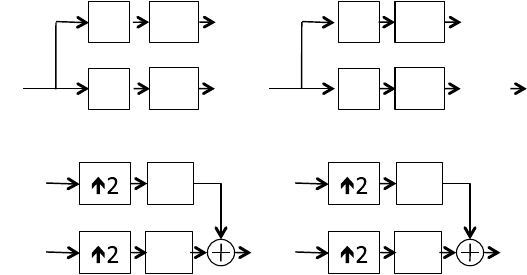
Progressive Data Access for Regular Grids 157
sequence of bands. By downsampling the results of each convolution, the total
number of non-zero coefficients is held constant through each pass.
(a)
(b)
FIGURE 8.3: The analysis of the input signal, c
j
, is performed by a cascade
of convolutions, followed by downsampling steps in (a). Reconstruction of c
j
is performed by a cascade of upsampling, followed by convolution steps in a
process known as synthesis in (b).
A reconstructed signal, ˆc
j,k
, is obtained with the Inverse Discrete Wavelet
Transform (IDWT) in a process known as synthesis,where,
ˆc
j,k
=
n
g
0
[k − 2n]c
j−1
[n]+g
1
[k − 2n]d
j−1
[n]. (8.20)
Analogous to Equations 8.18 and 8.19, the IDWT is equivalent to up-
sampling c
j
and d
j
by the introduction of zeros in every other sample and
summing the convolutions of c
j
and d
j
with g
0
and g
1
, respectively, as illus-
trated in Figure 8.3b. To ensure that ˆc
j,k
= c
j,k
, the inverse transform must
exhibit the property of perfect reconstruction. The reconstruction filters, g
0
and g
1
, must be chosen accordingly. But how does one know that g
0
and g
1
even exist? Conveniently, for orthogonal filters the reconstruction (synthesis)
filters do exist and are related to the analysis filters by:
g
0
[n]=h
0
[n]=
˜
h
0
[N − n],
g
1
[n]=h
1
[n]=
˜
h
1
[N − n].
(8.21)
An obvious question that arises is this: Given a signal x[k], how are the
initial c
j
max
,k
computed? Fortunately, if the samples of x[k] are computed
above the Nyquist rate, it can be assumed that c
j
max
,k
≈ x[k].
158 High Performance Visualization
8.4.4 Compression
Now, all the machinery is in place to provide a multiresolution representa-
tion of a 1D sampled signal. The DWT transforms x[n] into a wavelet space
sequence of coefficients, c
j,k
and d
j,k
. From the wavelet space representation
there is a coarsened approximation of x[n]givenbyc
j=0
that can progressively
be refined by adding a resolution by way of Equation 8.20.
The real power of the wavelet transform comes from the aforementioned
ability of wavelets to concentrate energy into a small number of coefficients.
Assume a discrete signal, x[n], expressed as the expansion
x[n]=
K−1
k=0
a
k
u
k
[n],
for some set of compactly supported basis functions u
k
. The goal is to find an
approximation of x[n], such that,
˜x[n]=
˜
K−1
k=0
˜a
k
u
k
[n],
where
˜
K<K. Moreover, for a given
˜
K, it is desired that the approximation
˜x[n] to be the best possible approximation for x[n] by some error metric. One
possibility is ||x[n] − ˜x[n]||
p
<for some norm, p. For an orthonormal basis,
for p =2,
||x[n] − ˜x[n]||
2
2
=
K−1
k=
˜
K
(a
π(k)
)
2
, (8.22)
where π(k)isapermutationof0...K − 1 such that
|a
π(0)
|≥...≥|a
π(K−1)
|,
and ˜x uses the coefficients corresponding to the first
˜
K − 1elementsofπ(k).
Formally:
˜a
k
=
a
k
if π(k) <
˜
K,
0 otherwise.
Thus, the L
2
error of ˜x[n]isgivenbythesumofthesquareofthecoefficients
a[k] that are not included in the expansion of ˜x[n]. To minimize the L
2
error for
agiven
˜
K, a
k
is sorted by decreasing the magnitude and only the
˜
K −1 largest
coefficients are included in the approximation. Alternatively, if a particular
is wanted, Equation 8.22 allows the calculation of how many and which
coefficients can be discarded to ensure ||x[n] − ˜x[n]||
p
<. Note, for any
a[k] = 0 its exclusion introduces no error in the approximation.
Progressive Data Access for Regular Grids 159
Equation 8.22 sheds some light on the choice of wavelet. As discussed ear-
lier (see Eq. 8.17), a wavelet possessing a higher number of vanishing moments
will permit the compaction of more energy (information) into fewer expansion
coefficients. Figure 8.4 qualitatively compares the compression of a signal by
a factor of 8, by using wavelets with different numbers of vanishing moments.
For ease of comparison, Figures 8.4a and 8.4b reproduce Figures 8.2a and 8.2b,
respectively. Results using the Haar (Fig. 8.4c) and Daubechies D4 (Fig. 8.4d)
wavelet are shown with one and two vanishing moments, respectively. Note
the “blockiness” resulting from the box shape of the Haar wavelet. Also note
that while the multiresolution approximation of Figure 8.4b may appear vi-
sually more appealing than Figure 8.4c, many extreme values in the original
signal are lost, which is the result of the cascade of applications of the low-pass
scaling filter.
Finally, unlike the pure multiresolution approaches based on Z-order curve
and wavelets, an arbitrary number of approximations are now produced. In
the extreme case, the approximation is refined one coefficient at a time.
8.4.5 Boundary Handling
Finite length signals present a couple of challenges that have been ignored
until this point. Consider the application of the DWT to a signal x[n]witha
low-pass filter h of length L = 4. By Equation 8.18, the computation of c[0]
is given by
c[0] =
˜
h[3]x[−3] +
˜
h[2]x[−2] +
˜
h[1]x[−1] +
˜
h[0]x[0].
But, for a finite signal, the samples x[−3], x[−2], and x[−1] do not exist! One
simple solution is to extend x[n] so that it is defined for n<0andn ≥ N.
There are a number of choices for the extension values, such as zero padding
or repeating the boundary samples, each with its own set of trade-offs. In the
general case, however, if the input signal, x, is extended, creating a new input
signal, x
e
of length N
e
>N, the resulting output after filtering and downsam-
pling no longer has exactly N non-zero and non-redundant approximations
and detail coefficients. Moreover, perfect reconstruction of x
e
requires all of
the N
e
coefficients. Due to downsampling in the case of the DWT, each iter-
ation of the filter bank requires an extension of the incoming approximation
coefficients. For a 1D signal, this overhead may not be significant, but later,
when moving on to 2D and 3D grids, the additional coefficients can consume
a substantial amount of space.
A filter bank that is nonexpansive is more preferable, as it preserves the
number of input coefficients on output, and does not introduce discontinuities
at the boundaries. The solution is the employment of symmetric filters com-
bined with a symmetric signal extension. Only the case of signals of length
N =2
n
, and odd length filters where the symmetry is about the center bound-
ary coefficients, is considered here. For an extensive discussion on symmetric
..................Content has been hidden....................
You can't read the all page of ebook, please click here login for view all page.