

160 High Performance Visualization
0
2
00
4
00 600 800
1
000
−80
−60
−40
−20
0
20
40
60
(a)
0
2
0
4
0 60 80
1
00
12
0
−80
−60
−40
−20
0
20
40
60
(b)
0
2
00
4
00 600 800
1
000
−80
−60
−40
−20
0
20
40
60
(c)
0
2
00
4
00 600 800
1
000
−80
−60
−40
−20
0
20
40
60
(d)
FIGURE 8.4: A test signal (a) with 1024 samples and a multiresolution ap-
proximation, (b), at 1/8
th
resolution, reproduced from Figure 8.2. The test
signal reconstructed using 1/8
th
of the expansion coefficients with the largest
magnitude from the Haar, (c), and Daubechies 4-tap wavelet, (d), respectively.
Progressive Data Access for Regular Grids 161
filters of even length, which introduce considerably more complexity, or han-
dling N =2
n
(see [1, 12]). For clarity of exposition, assume that the filter
is whole-sample symmetric about h[0]. That is, h[n]=h[−n], and h[0] is not
repeated. For example, if L = 3, the center point is h[0], and h[−1] = h[1].
Moreover, the input signal must be made a whole-sample symmetric about the
first (n =0)andlast(n = N −1) samples. The motivation for this symmetry
is straightforward: the output samples for n<0andn ≥ N are redundant
and need not be explicitly stored. Consider the calculation in a general lin-
ear transform of the expansion coefficient a[−1], by the convolution of x with
h[−n] for whole-sample symmetric x,andh,withL =3:
a[−1] = h[0]x[−2] + h[1]x[−1] + h[2]x[0].
Due to symmetry, h[n]=h[−n], and x[n]=x[−n]. Therefore:
a[1] = a[−1] = h[0]x[2] + h[1]x[1] + h[2]x[0],
and a[−1] is redundant and need not be explicitly stored!
Things become a little more complicated with the DWT, which operates as
a dual channel convolution filter, followed by downsampling. Here, centering
the filter must be done carefully for each channel, such that symmetry is
preserved after downsampling, and the total number of coefficients output by
the two channels, equals the number of input coefficients. For even N , each
channel outputs exactly N/2 samples.
Symmetric filters combined with a symmetric signal extension provide a
straightforward mechanism for dealing with finite length signals and the DWT.
Unfortunately, with the exception of the Haar wavelet, there are no orthogonal
wavelets with compact support possessing both the property of symmetry and
perfect reconstruction. The solution to this dilemma is the relaxation of the
orthogonality requirement and the introduction of biorthogonal wavelets. For
biorthogonal wavelets, the properties of Equation 8.11 no longer hold. Differ-
ent analysis scaling and wavelet basis functions,
˜
φ(t)and
˜
ψ(t), and synthesis
scaling and wavelet basis, φ(t)andψ(t), must be introduced. Similarly, new
analysis,
˜
h
0
and
˜
h
1
, and synthesis filters, g
0
and g
1
, will appear.
From a filter bank perspective, h
1
no longer relates to h
0
by a simple
expression. However, the following cross relationship between synthesis and
analysis filters hold:
˜
h
0
[n]=(−1)
n
g
1
(N − 1 − n),g
0
[n]=(−1)
n
˜
h
1
(N − 1 − n), (8.23)
where N is the support size of the filter.
With the analysis filters no longer related to each other by Equation 8.15,
the support of these respective filters need not be the same. The support sizes
of
˜
h
0
and
˜
h
1
are then denoted as L
0
and L
1
, respectively, leading to new
analysis equations:
162 High Performance Visualization
c
j,k
=
(L
0
−1)/2
n=−(L
0
−1)/2
˜
h
0
[n]c
j+1
[2k − n], (8.24)
d
j,k
=
(L
1
−1)/2
n=−(L
1
−1)/2
˜
h
1
[n]c
j+1
[2k − n +1]. (8.25)
Note that Equation 8.24 processes the even samples of c
j+1
, while Equa-
tion 8.25 processes the odd samples—a necessity for nonexpansive output [12].
Because of the shift in the inputs to the analysis equation, a new synthesis
equation is also necessary, which must shift the d[n]coefficients:
ˆc
j,k
=
n
g
0
[k − 2n]c
j−1
[n]+g
1
[k − 2n − 1]d
j−1
[n]. (8.26)
As already noted, the correct behavior of Equations 8.24 and 8.25 is pred-
icated on treating the input signal, c
j+1
[n], as exhibiting whole-sample sym-
metry about the left and right boundary. Perfect reconstruction from Equa-
tion 8.26 requires a mixture of whole-sample and half-sample symmetry, where
the point of symmetry lies halfway between two samples. Signals with the left
boundary, half-sample symmetry are symmetric about the non-integer point
−
1
2
, while right boundary, half-sample symmetric signals are symmetric about
the point N −
1
2
—for the left boundary, x[−1] = x[0], x[−2] = x[1] and so on.
For Equation 8.26, the left and right boundaries of c[n]andd[n] must be made
whole-sample symmetric, respectively, while the right and left boundaries of
c[n]andd[n] must be half-sample symmetric, respectively. Lastly, for both
the symmetric analysis filters,
˜
h
0
[n]and
˜
h
1
[n], and the symmetric synthesis
filters, g
0
[n] and g
1
[n], the filters have a zero value for n<(L − 1)/2and
n>(L − 1)/2, where L is the support size of the filter.
Although symmetry is gained and the number of inputs and output are
preserved, by giving up orthogonality, other important properties are lost.
Most significantly, Equation 8.22 no longer holds, and the L
2
error between
asignalx and its approximation ˜x can no longer be determined by the co-
efficients (not included in the construction of ˜x). Nevertheless, the L
2
error,
introduced in the reconstruction after discarding coefficients, is still minimized
by discarding the coefficients of smallest magnitude.
Figure 8.5 shows plots of the Cohen-Daubechies-Feauveau (CDF) 9/7
biorthogonal synthesis and the analysis functions. Note the symmetry in all
of the functions. Table 8.1 provides the filter coefficients for the CDF 5/3 and
9/7 normalized, biorthogonal wavelets. These filters are the foundation for
the JPEG2000 image compression standard. The reader is cautioned that the
naming of the CDF family of biorthogonal wavelets is inconsistent in the liter-
ature. Here, the naming convention based on the support size in the low-pass
analysis and synthesis filters, respectively (e.g., CDF 9/7), is adopted. Other
authors use a naming scheme based on the number of analysis and synthesis
filter vanishing moments, respectively (e.g., bior4.4).

Progressive Data Access for Regular Grids 163
0 500
1
000
1
500
2
000
−0.5
0
0.5
1
1.5
(a)
0 500
1
000
1
500
2
000
−2
−1
0
1
2
(b)
0 500
1
000
1
500
2
000
−0.5
0
0.5
1
1.5
(c)
0 500
1
000
1
500
2
000
−0.5
0
0.5
1
1.5
(d)
FIGURE 8.5: The CDF 9/7 biorthogonal wavelet and scaling functions: analy-
sis scaling (a) and wavelet functions (b), and synthesis scaling (c) and wavelet
functions (d).
TABLE 8.1: Biorthogonal wavelet filter coefficients for the CDF 5/3 (top) and
9/7 (bottom) wavelets
pn h
0
[n] g
0
[n]
2 0 1.06066017177982 0.70710678118655
−1, 1 0.35355339059327 0.35355339059327
−2, 2 -0.17677669529663 0
4 0 0.852698679008894 0.788485616405583
−1, 1 0.377402855612831 0.418092273221617
−2, 2 -0.110624404418437 -0.0406894176091641
−3, 3 -0.023849465019557 -0.0645388826286971
−4, 4 0.037828455507264 0.0
164 High Performance Visualization
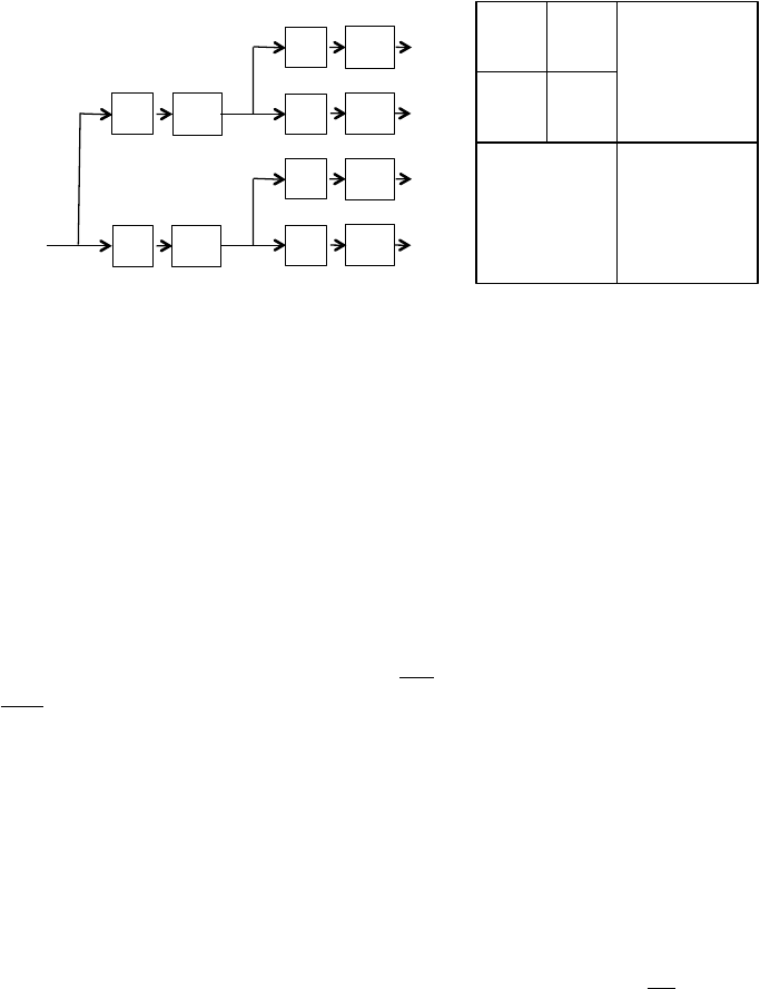
(a)
(b)
FIGURE 8.6: On the left, (a) shows a single pass of the 2D DWT resulting
in one set of approximation coefficients, and three sets of detail coefficients.
The right side of the figure (b) shows the resulting decomposition after two
passes of the DWT. As each coefficient is the result of two filtering steps, one
along each dimension, the superscripts in (a) and (b) indicate highpass, H,or
lowpass, L, filtering.
8.4.6 Multiple Dimensions
Extending the 1D wavelet filter bank to multiple dimensions is straight-
forward. The 1D analysis filter is simply applied along each dimension is il-
lustrated in the 2D example in Figure 8.6. Thus, for a M × N grid, a single
pass of the 2D DWT yields, on average
MN
4
approximation coefficients and
3MN
4
detail coefficients. For 3D data, seven times as many detail coefficients
as approximation coefficients are generated for each iteration of the DWT.
8.4.7 Implementation Considerations
There are two possible approaches used to construct a PDA model, based
on the forward and inverse DWT. A multiresolution hierarchy can be con-
structed, just like with the Z-order space-filling curve, and by exposing the
scale parameter, j, in Equation 8.10 the grid may be coarsened or refined
by factors of 2
d
. This approach is called frequency truncation. Each iteration
of the analysis filters uses the normalized coefficients provided in Table 8.1,
which scales the amplitude of the approximation coefficients by
√
2.0. If the
approximation coefficients are used as an approximation of the original sig-
nal, this scaling should be undone by multiplication by 2
−1/j
,wherej is the
number of iterations of the analysis filter. Alternatively, the wavelet expansion
representation’s power can be exploited to concentrate most of a signal’s infor-
mation content into a small number of expansion coefficients. This approach
..................Content has been hidden....................
You can't read the all page of ebook, please click here login for view all page.