
Chapter 10
Streaming and Out-of-Core Methods
David E. DeMarle
Kitware Inc.
Berk Geveci
Kitware Inc.
Jon Woodring
Los Alamos National Laboratory
Jim Ahrens
Los Alamos National Laboratory
10.1 External Memory Algorithms .................................... 200
10.2 Taxonomy of Streamed Visualization ............................ 202
10.3 Streamed Visualization Concepts ................................ 204
10.3.1 Data Structures .......................................... 204
10.3.2 Repetition ............................................... 205
10.3.3 Algorithms ............................................... 205
10.3.4 Sparse Traversal ......................................... 206
10.4 Survey of Current State of the Art .............................. 209
10.4.1 Rendering ................................................ 209
10.4.2 Streamed Processing of Unstructured Data ............. 210
10.4.3 General Purpose Systems ................................ 211
10.4.4 Asynchronous Systems .................................. 212
10.4.5 Lazy Evaluation ......................................... 214
10.5 Conclusion ........................................................ 215
References .......................................................... 216
One path toward visualizing ever-larger data sets is to use external memory or
out-of-core (OOC) algorithms. OOC algorithms are designed to process more
data than can be resident in the main memory at any one time, and the OOC
algorithms do this by optimizing external memory transfers.
Even if only within a pre-processing phase, OOC algorithms run through
the entire data, processing some portion, and then freeing up space before
moving on to the next portion. Streaming is the concept of piecemeal data
processing and applying some computation kernel on each portion. In this way,
199
200 High Performance Visualization
managing the memory footprint directly addresses the large data challenge
and it can also improve performance, even on small data because of the effect
of forced locality of data references on the memory hierarchy [32, 9, 34, 40].
However, there are challenges to applying streaming in general purpose
visualization. Some data structures are not well-suited for partitioning, and
not every algorithm can work within the confines of a restricted portion of the
data. Also, since a streaming formulation of an algorithm may involve many
passes through the data where each pass can be time consuming, optimizations
are essential for interactive data exploration. Fortunately, given that the data
is to be processed in distinct portions, streaming facilitates skipping (culling)
unimportant portions of the data, which can amount to a majority of the
input.
This chapter first discusses OOC processing and streaming, in general.
First, it considers the design parameters for applying the concept of stream-
ing to scientific visualization. Second, it presents some observations on the
potential optimizations and hazards of doing scientific visualization within
a streaming framework. With an appreciation of these fundamentals, recent
works are surveyed in which the streaming concept plays an important part
of the implementation. The discussion will conclude by summarizing the state
of the art and a conjecture about the future.
10.1 External Memory Algorithms
The most popular approach to large data visualization is data parallelism.
In data parallelism, the system takes advantage of the aggregate memory
of a set of processing elements by splitting up the data among all of them.
Each processing element only computes the portion for which it is responsible.
Chapters 16, 18, and 21 describe current scientific visualization systems that
make use of data parallelism.
Data parallelism implicitly assumes that the data fits entirely in a large ag-
gregate memory space, somewhere. Getting access to a large enough memory
space can be expensive and otherwise impractical for many users. Streaming
exchanges resources for time—instead of using ten machines to visualize a
problem, one machine might visualize the same problem but take ten times
longer. Streaming then allows all users to process larger data sets than they
otherwise could, regardless of the size of the machine.
External memory algorithms are written with the assumption that the
entire problem cannot be loaded all at once. These algorithms are described
well in surveys by Vitter [35], Silva [31], and Lipsa [22]. Vitter first classi-
fied external memory algorithms into two groups: online problems and batch
problems.
Online problems deal with large data by first pre-processing data and then
making queries into an organized whole, out of which each query can be sat-
isfied by touching only a small portion. The data structures and algorithms
Streaming and Out-of-Core Methods 201
portion
1
portion
2
portion
3
portion
1
done
portion
2
portion
3
waiting
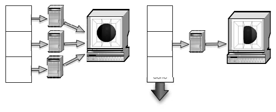
FIGURE 10.1: A comparison of data parallel visualization and streaming.
used are designed so that they never overflow the available RAM, and they re-
quire as few slow external memory accesses as possible by amortizing the cost
of each access across many related data items. Pre-processing is very effective
for visualization because typically only a small fraction of the total data con-
tributes to a meaningful visualization [9]. For example, a pre-processing step
can sort or index the data by data values to help accelerate thresholding and
isocontouring operations.
Since scientific visualization presents the results to the user in a graph-
ical format, the user can also take advantage of the numerous techniques
developed for rendering. If data is spatially sorted into coherent regions, large
areas can be skipped, and screen space appropriate details quickly rendered.
iWalk [8], an interactive walkthrough system, does this by using an OOC sort-
ing algorithm to build an octree on a disk containing scene geometry in the
nodes. At runtime, visible nodes are determined and fetched (speculatively)
by a thread that runs asynchronously from the rendering. Likewise, many
level-of-detail systems [28, 13] compute summary information during the pre-
processing stage; they later fetch that information from a disk and render
approximations while the user interacts and whenever the full-resolution data
covers too few pixels for full details to be seen. To be fully scalable, the algo-
rithm must be end-to-end out-of-core, meaning that neither the runtime nor
the pre-processing phases allow the data to exceed the available RAM.
Batch problems operate by iterating through the data one time or many
times, touching only a small portion of the large data at any given time, and
then accumulating or writing out new results as they are generated, until
completion. These algorithms are most often called “streamed” processing in
visualization. This helps to eliminate confusion with the more typical meaning
of “batch,” producing visualizations in unattended sessions.
In a survey of stream processing within the wider field of computer science,
Stephens shows that the streaming concept has been used since at least the
1960s [33]. Within his framework of stream processing systems, data flow
networks hold the greatest amount of interest, since they are the dominant

202 High Performance Visualization
Stream Length Fixed or unbounded data set size.
Partition Axes Temporal, geometric, topological, other.
Granularity Block, subblock, cell.
Route What holds the whole data and what processes
it a chunk at a time.
Asynchrony Can chunks be processed simultaneously?
TABLE 10.1: Taxonomy of streaming.
architecture for constructing general purpose visualization programs today.
This chapter primarily focuses on data flow visualization systems.
Stream processing has been used within visualization for decades as
well [14, 32]. Law et al. [21] added a streaming framework to a general purpose
scientific visualization library, the Visualization Toolkit (VTK) [30], and later
to its sister toolkit, the Insight Toolkit (ITK) [15]. In their streaming frame-
work, a series of pipeline passes allow filters to negotiate how a structured
data set is split into memory size-limited portions called pieces. In the first
pass the network determines the overall problem domain. In the next pass, the
network prepares to visualize one specific piece. Next, the pipeline runs fully
to produce a visualization of that piece. In this way, each piece is processed,
in turn, by all filters along the visualization pipeline.
As illustrated in Figure 10.1, there is a strong relationship between stream-
ing and data parallel processing. If the data can be processed in portions, many
portions could be processed simultaneously. In later work, the same architec-
ture is used as the basis for data parallel visualization within VTK [1]. The
two techniques are in fact complementary and can be combined.
10.2 Taxonomy of Streamed Visualization
In general, it is assumed that streamed visualization is the processing and
rendering of a sequence of data values, which in turn, will only keep a portion
of the whole data set in memory at any given time. Under this assumption,
streaming algorithms are parameterized by the contents of the stream, how
the data is ordered, how long the stream is, and how exactly it is processed.
Under this classification, a taxonomy of streaming is described within scientific
visualization.
One axis of the taxonomy is whether the stream is of fixed or unbounded
length. Consider the case of operating on an endless stream, as is the case in
signal processing frameworks. An analogy within the visualization community
is in situ visualization. As explained in Chapter 9 with in situ visualization,
the visualization engine computes graphical results as data are generated or
obtained. When the visualization program purges old values to keep memory
usage bounded, this is a form of streaming.

Streaming and Out-of-Core Methods 203
portion
1
done
portion
2
starting
portion
3
waiting
portion 1
portion 3
portion 2
portion 1
contour
read
render
portion
1
done
portion
2
working
portion
3
working
contour
read
render
FIGURE 10.2: Synchronous (left) and asynchronous (right) streaming in a
data flow visualization network.
The second axis of the taxonomy is which axes the data is divided along:
spatial, temporal, topological, or some combination of these. Most time-
varying simulations produce a new data set that covers the entire spatial
domain at each computed timestep. It is almost always impractical to store
all of the time slices in memory at once, so visualization of time-varying data
is almost always streamed. Streaming through the timesteps works because
many visualization algorithms require only one or a few timesteps to be loaded
at once [24, 4]. Still, in many cases, a single timestep is too large to fit into the
memory all at once, therefore, the data is partitioned in the spatial domain
as well.
The third axis is the granularity by which the data is divided. The largest
possible portion size is just smaller than the available memory of the machine
and the smallest is the size of an individual data item. There are computational
trade-offs though, with respect to the level of granularity [9, 37, 2]. Smaller
portions make a better utilization of cache architectures and allow sparse data
traversal to skip over more of the data that ultimately does not contribute to
the visualization. Larger portion sizes do not force the visualization system to
update as many times to cover the same space.
The fourth axis is the path that data takes as it is streamed. So far, the
cases being discussed are the case of streaming data off a disk, through a
visualization algorithm and onto the screen. However, streaming also includes
the case in which data is too large for a local disk, and therefore, it is acquired
from a server and processed locally, one portion at a time [9, 29, 20]. Likewise,
streaming applies when data is streamed to and processed within a GPU.
The fifth axis of the taxonomy is the degree of asynchrony within the
visualization system. Once data is partitioned, a system may allow different
portions to be processed simultaneously. For example, in a client–server frame-
work, the client might display some results while the server fetches additional
portions for it to process. As another example, the modules within a visualiza-
tion pipeline can operate as a staged parallel pipeline [32, 1, 34, 36] if there is
..................Content has been hidden....................
You can't read the all page of ebook, please click here login for view all page.