

296 High Performance Visualization
7LPHV
&RUHV
3XUSOH
&RUHV
'DZQ
&RUHV
-XQR
&RUHV
5DQJHU
&RUHV
)UDQNOLQ
&RUHV
-DJXDU3)
,2
&RQWRXU
5HQGHU
FIGURE 13.2: Plots of execution time for the I/O, contouring, and rendering
phases of the trillion cell visualizations over six supercomputing environments.
I/O was by far the slowest portion. Image source: Childs et al., 2010 [1].
13.2.1 Varying over Supercomputing Environment
The first variant of the experiment was designed to understand differences
from supercomputing environment. The experiment consisted of running an
identical problem on multiple platforms, keeping the I/O pattern and data
generation fixed, and using noncollective I/O and upsampled data generation.
Results can be found in Figure 13.2 and Table 13.2.
Machine Cores Data set size I/O Contour TPE Render
Purple 8000 0.5 TCells 53.4s 10.0s 63.7s 2.9s
Dawn 16384 1 TCells 240.9s 32.4s 277.6s 10.6s
Juno 16000 1 TCells 102.9s 7.2s 110.4s 10.4s
Ranger 16000 1 TCells 251.2s 8.3s 259.7s 4.4s
Franklin 16000 1 TCells 129.3s 7.9s 137.3s 1.6s
JaguarPF 16000 1 TCells 236.1s 10.4s 246.7s 1.5s
Franklin 32000 2 TCells 292.4s 8.0s 300.6s 9.7s
JaguarPF 32000 2 TCells 707.2s 7.7s 715.2s 1.5s
TABLE 13.2: Performance across diverse architectures. “TPE” is short for
total pipeline execution (the amount of time to generate the surface). Dawn’s
number of cores is different from the rest since that machine requires all jobs
to have core counts that are a power of two.
There were several noteworthy observations:
• I/O striping refers to transparently distributing data over multiple disks
to make them appear as a single fast, large disk; careful consideration
of the striping parameters was necessary for optimal I/O performance
on Lustre filesystems (Franklin, JaguarPF, Ranger, Juno, & Dawn).
Even though JaguarPF had more I/O resources than Franklin, its I/O
Visualization at Extreme Scale Concurrency 297
performance did not perform as well in these experiments, because its
default stripe count was four. In contrast, Franklin’s default stripe count
of two was better suited for the I/O pattern which read ten separate
compressed files per task. Smaller stripe counts often benefit file-per-
task I/O because the files were usually small enough (tens of MB) that
they would not contain many stripes, and spreading them thinly over
many I/O servers increases contention.
• Because the data was stored on disk in a compressed format, there was
an unequal I/O load across the tasks. The reported I/O times measure
the elapsed time between a file open and a barrier, after all the tasks
were finished reading. Because of this load imbalance, I/O time did not
scale linearly from 16,000 to 32,000 cores on Franklin and JaguarPF.
• The Dawn machine has the slowest clock speed (850MHz), which was
reflected in its contouring and rendering times.
• Some variation in the observations could not be explained by slow clock
speeds, interconnects, or I/O servers:
– For Franklin’s increase in rendering time from 16,000 to 32,000
cores, seven to ten network links failed that day and had to be
statically re-routed, resulting in suboptimal network performance.
Rendering algorithms are “all reduce” type operations that are very
sensitive to bisection bandwidth, which was affected by this issue.
– The experimenters concluded Juno’s slow rendering time was sim-
ilarly due to a network problem.
13.2.2 Varying over I/O Pattern
This variant was designed to understand the effects of different I/O pat-
terns. It compared collective and noncollective I/O patterns on Franklin for
a one trillion cell upsampled data set. In the noncollective test, each task
performed ten pairs of fopen and fread calls on independent gzipped files
without any coordination among tasks. In the collective test, all tasks syn-
chronously called MPI
File open once, then called MPI File read at all ten
times on a shared file (each read call corresponded to a different piece of the
data set). An underlying collective buffering, or “two phase” algorithm, in
Cray’s MPI-IO implementation aggregated read requests onto a subset of 48
nodes (matching the 48 stripe count of the file) that coordinated the low-level
I/O workload, dividing it into 4MB stripe-aligned fread calls. As the 48 ag-
gregator nodes filled their read buffers, they shipped the data using message
passing to their final destination among the 16,016 tasks. A different number
of tasks was used for each scheme (16,000 versus 16,016), because the collec-
tive communication scheme could not use an arbitrary number of tasks; the
298 High Performance Visualization
closest value to 16,000 possible was picked. Performance results are listed in
Table 13.3.
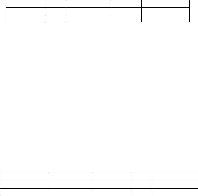
I/O pattern Cores Total I/O time Data read Read bandwidth
Collective 16016 478.3s 3725.3GB 7.8GB/s
Noncollective 16000 129.3s 954.2GB 7.4GB/s
TABLE 13.3: Performance with different I/O patterns. The bandwidth for
the two approaches are very similar. The data set size for collective I/O cor-
responds to four bytes for each of the one trillion cells. The data read is
less than 4000GB because, 1GB is 1,073,741,824 bytes. The data set size for
noncollective I/O is much smaller because it was compressed.
Both patterns led to similar read bandwidths, 7.4 and 7.8GB/s, which are
about 60% of the maximum available bandwidth of 12GB/s on Franklin. In the
noncollective case, load imbalances, caused by different compression factors,
may account for this discrepancy. For the collective I/O, coordination overhead
between the MPI tasks may be limiting efficiency. Of course, the processing
would still be I/O dominated, even if perfect efficiency was achieved.
13.2.3 Varying over Data Generation
This variant was designed to understand the effects of source data. It
compared upsampled and replicated data sets, with each test processing one
trillion cells on 16,016 cores of Franklin using collective I/O. Performance
results are listed in Table 13.4.
Data generation Total I/O time Contour time TPE Rendering time
Upsampling 478.3s 7.6s 486.0s 2.8s
Replicated 493.0s 7.6s 500.7s 4.9s
TABLE 13.4: Performance across different data generation methods. “TPE” is
short for total pipeline execution (the amount of time to generate the surface).
The contouring times were nearly identical, likely since this operation is
dominated by the movement of data through the memory hierarchy (L2 cache
to L1 cache to registers), rather than the relatively rare case where a cell
contains a contribution to the isosurface. The rendering time, which is pro-
portional to the number of triangles in the isosurface, nearly doubled, because
the isocontouring algorithm run on the replicated data set produced twice as
many triangles.
Visualization at Extreme Scale Concurrency 299
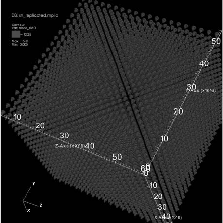
FIGURE 13.3: Contouring of replicated data (one trillion cells total), visual-
ized with VisIt on Franklin using 16,016 cores. Image source: Childs et al.,
2010 [1].
13.3 Scaling Experiments
Where the first part of the experiment [1] informed performance bottle-
necks of pure parallelism at an extreme scale, the second part sought to assess
its weak scaling properties for both isosurface generation and volume render-
ing. Once again, these algorithms exercise a large portion of the underlying
pure parallelism infrastructure and indicates a strong likelihood of weak scal-
ing for other algorithms in this setting. Further, demonstrating weak scaling
properties on high performance computing systems met the accepted stan-
dards of “Joule certification,” which is a program within the U.S. Office of
Management and Budget to confirm that supercomputers are being used effi-
ciently.
13.3.1 Study Overview
The weak scaling studies were performed on an output from Denovo, which
is a 3D radiation transport code from ORNL that models radiation dose levels
in a nuclear reactor core and its surrounding areas. The Denovo simulation
code does not directly output a scalar field representing effective dose. Instead,
this dose is calculated at runtime through a linear combination of 27 scalar
fluxes. For both the isosurface and volume rendering tests, VisIt read in 27
300 High Performance Visualization
scalar fluxes and combined them to form a single scalar field representing
radiation dose levels. The isosurface extraction test consisted of extracting six
evenly spaced isocontour values of the radiation dose levels and rendering an
1024 × 1024 pixel image. The volume rendering test consisted of ray casting
with 1000, 2000 and 4000 samples per ray of the radiation dose level on a
1024 × 1024 pixel image.
These visualization algorithms were run on a baseline Denovo simulation
consisting of 103,716,288 cells on 4,096 spatial domains, with a total size on
disk of 83.5GB. The second test was run on a Denovo simulation nearly three
times the size of the baseline run, with 321,117,360 cells on 12,720 spatial
domains and a total size on disk of 258.4GB. These core counts are large rela-
tive to the problem size and were chosen because they represent the number of
cores used by Denovo. This matching core count was important for the Joule
study and is also indicative of performance for an in situ approach.
13.3.2 Results
Tables 13.5 and 13.6 show the performance for contouring and volume ren-
dering respectively, and Figures 13.4 and 13.5 show the images they produced.
The time to perform each phase was nearly identical over the two concurrency
levels, which suggests the code has favorable weak scaling characteristics. Note
that I/O was not included in these tests.
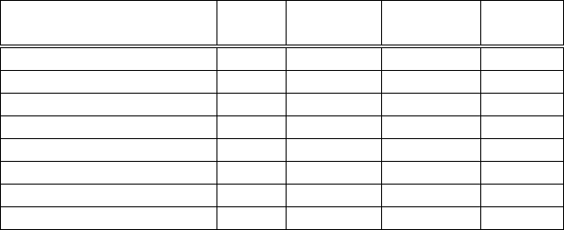
Algorithm Cores Minimum Maximum Average
Time Time Time
Calculate radiation 4,096 0.18s 0.25s 0.21s
Calculate radiation 12,270 0.19s 0.25s 0.22s
Isosurface 4,096 0.014s 0.027s 0.018s
Isosurface 12,270 0.014s 0.027s 0.017s
Render (on task) 4,096 0.020s 0.065s 0.0225s
Render (on task) 12,270 0.021s 0.069s 0.023s
Render (across tasks) 4,096 0.048s 0.087s 0.052s
Render (across tasks) 12,270 0.050s 0.091s 0.053s
TABLE 13.5: Weak scaling study of isosurfacing. Isosurface refers to the
execution time of the isosurface algorithm, Render (on task) indicates the
time to render that task’s surface, while Render (across tasks) indicates
the time to combine that image with the images of other tasks. Calculate
radiation refers to the time to calculate the linear combination of the 27
scalar fluxes.
..................Content has been hidden....................
You can't read the all page of ebook, please click here login for view all page.