

312 High Performance Visualization
(a) Synthetic, noisy data
set.
(b) Gaussian smoothing
(r = 16).
(c) Bilateral smoothing
(r = 16,σ = 15%).
FIGURE 14.1: These images compare the results of smoothing to a synthetic
data set (a), which contains added noise. While Gaussian smoothing blurs
the sharp edge in this data set (b), bilateral filtering removes noise (c), while
preserving the sharp edge. Image source: Bethel, 2009 [1].
an abrupt change in the signal. Figure 14.1 shows how bilateral filtering is
a preferable operation for anisotropic smoothing, in comparison to the tradi-
tional Gaussian filtering of a 3D, synthetic data set with added noise.
The bilateral filter kernel is a good candidate to use in a performance
optimization study on multi- and many-core platforms because it is quite
computationally expensive compared to other common stencil kernels, e.g.,
Laplacian, divergence, or gradient operators [16]. Also, the size of the stencil,
or bilateral filter window, varies according to its user preference and appli-
cation, whereas most other stencil-based solvers tend to consider only the
nearest-neighbor points.
The subsections that follow present a summary of a study by Bethel [2].
The study reports there can be as much as a 7.5× performance gain possible,
depending on the setting of one tunable algorithmic parameter for a given
problem on a given platform, and an additional 4× gain possible, through a
combination of algorithmic optimizations and the use of device-specific capa-
bilities, for a total of about a 30× the overall possible performance gain.
14.2.2 Design and Methodology
The main focus of this study is to examine how an algorithmic design
option, a device-specific feature, and one tunable algorithmic parameter can
combine to produce the best performance. The algorithmic design choice tells
how to structure the CUDA implementation inner loop of the 3D bilateral
filter so as to iterate over the voxels in memory (see 14.2.3.1). The device-
specific feature makes use of local, high-speed memory for storing filter weights
so as to avoid recomputing them over and over again. These filter weights
remain constant for the course of each problem run (see 14.2.3.2). Finally,

Performance Optimization and Auto-Tuning 313
%FQUI3PX
8JEUI3PX
)FJHIU3PX
(a) Three potential thread memory access
patterns: depth-, width-, and height-row.
$EVROXWH5XQWLPHRI7KUHH'LIIHUHQW0HPRU$FFHVV3DWWHUQV
)LOWHU5DGLXV
([HFXWLRQ7LPHPV
'HSWK5RZ
:LGWK5RZ
+HLJKW5RZ
(b) Runtime performance for each of the
depth-, width-, and height-row traversals.
FIGURE 14.2: Three different 3D memory access patterns, (a) have markedly
different performance characteristics on a many-core GPU platform (b), where
the depth-row traversal is the clear winner by a factor of about 2×. Image
source: Bethel, 2009 [1].
the tunable algorithmic parameter is the size and shape of the CUDA thread
block (see 14.2.3.3).
14.2.3 Results
14.2.3.1 Algorithmic Design Option: Width-, Height-, and Depth-
Row Kernels
One of the first design choices in any parallel processing algorithm is to
decide on a work partitioning strategy. For this particular problem, there are
many potential partitionings of workload: they all come down to deciding how
to partition the 3D volume into smaller pieces that are assigned to different
processors.
In this particular study, the authors aim was to determine the memory ac-
cess pattern that yields the best performance. To that end, they implemented
three different memory access strategies. The first, called depth-row process-
ing, has each thread process all voxels along all depths for a given (i,j,*)
location. This approach appears as the dark, solid line and arrow on the 3D
grid shown in Figure 14.2a. A width-row order has each thread process all
voxels along a width at a given (*,j,k) location, and appears as a light gray,
solid line and arrow in Figure 14.2a. Similarly, a height-row traversal has each
thread process all voxels along a height at a given (i,*,k) location, and this
is shown as a medium-gray, dashed line and arrow in Figure 14.2a.
The results of the memory access experiment, shown in Figure 14.2b, in-
dicate the depth-row traversal offers the best performance by a significant
amount, about a 2× performance gain. The best performance stems from
the depth-row algorithm’s ability to achieve so-called “coalesced memory” ac-
314 High Performance Visualization
cesses. In the case of the depth-row algorithm, each of the simultaneously
executing threads will be accessing source and destination data that differs by
one address location, e.g., contiguous blocks of memory. The other approaches,
in contrast, will be accessing source and destination memory in noncontigu-
ous chunks. The performance penalty for non-contiguous memory accesses is
apparent in Figure 14.2b.
By simply altering how an algorithm iterates through memory, this re-
sult shows a significant impact on performance. Furthermore, this result will
likely vary from platform to platform, depending on the characteristics of the
memory subsystem. For example, different platforms have different memory
prefetch strategies, different sizes of memory caches, and so forth.
14.2.3.2 Device-Specific Feature: Constant Versus Global Memory
for Filter Weights
Another design consideration is how to take advantage of and leverage
device-specific features such as device memory types and memory speeds.
The NVIDIA GPU presents multiple types of memory, some slower and un-
cached, others faster and cached. According to the NVIDIA CUDA Program-
ming Guide [23], the amount of global (slower, uncached) and texture (slower,
cached) memory varies as a function of specific customer options on the graph-
ics card. Under CUDA v1.0 and higher, there is 64KB of constant memory
and 16KB of shared memory that resides on-chip and visible to all threads.
Generally speaking, device memory (global and texture memory) has a higher
latency and lower bandwidth than an on-chip memory (constant and shared
memories).
The authors wondered if storing, rather than recomputing, portions of the
problem in on-chip, high speed memory (a device-specific feature) would offer
any performance advantage. The portions of the problem they stored, rather
than recomputed, were the filter weights, which are essentially a discretization
of a 3D Gaussian and a 1D Gaussian function.
The performance question is then: “How is performance impacted by hav-
ing all of the filter weights resident in on-chip rather than in device memory?”
The results, shown in Figure 14.3, indicate that the runtime is about 2×
faster when the filter weights are resident in a high-speed, on-chip constant
memory, as opposed to when the weights reside in the device’s (slower) global
shared memory. This result is not surprising given the different latency and
bandwidth characteristics of the two different memory subsystems.
14.2.3.3 Tunable Algorithmic Parameter: Thread Block Size
In this particular problem, the tunable algorithmic parameter is the size
and shape of the CUDA thread block. The study’s objective is to find the
combination of block size parameters—a tunable algorithmic parameter—that
produce optimal performance.
A relatively simple example, shown in Figure 14.4, reveals that there is

Performance Optimization and Auto-Tuning 315
$EVROXWH3HUIRUPDQFH&RQVWDQWYV*OREDO0HPRU
)LOWHU5DGLXV
([HFXWLRQ7LPHPV
&RQVWDQW0HPRUDYJ
*OREDO0HPRUDYJ
(a) Absolute performance (smaller is
better).
5HODWLYH3HUIRUPDQFH&RQVWDQWYV*OREDO0HPRU
)LOWHU5DGLXV
([HFXWLRQ7LPHUHODWLYH
*OREDO0HPRUDYJ
&RQVWDQW0HPRUDYJ
(b) Relative performance (smaller is
better).
FIGURE 14.3: These results compare the absolute and relative performance
difference when precomputed filter weights are resident in device memory
vs. constant memory (2× faster). In all ranges of filter sizes, the constant
memory implementation performs about twice as fast as the device memory
implementation. Image source: Bethel, 2009 [1].
5XQWLPHIRU9DULQJ7KUHDG%ORFN6L]HVU
%ORFNVLQ;'LUHFWLRQ
%ORFNVLQ<'LUHFWLRQ
5XQWLPHPV
FIGURE 14.4: Runtime (ms) at radius r = 11 for different thread-block config-
urations on the GPU exhibit a 7.5× variation in performance: the coordinate,
(8, 128), has a runtime of 9,550 ms while (128, 128) is much slower at 71,537
ms. Image courtesy of Mark Howison (LBNL and Brown University).
uptoa7.5× performance difference between the best- and worst-performing
configurations for a filter radius width of r = 11, which corresponds to a
very large 23
3
-point stencil configuration.
1
The experiment varies the size of
1
A filter radius r corresponds to a filter “box size” of 2r + 1. So, a filter radius of 1
corresponds to a 3 × 3stencilin2D,ora3× 3 × 3 stencil in 3D.
316 High Performance Visualization
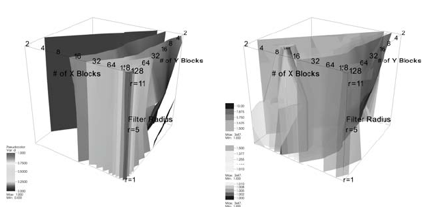
(a) Runtimes normalized by maximum
highlight the poorest performing configu-
rations.
(b) Runtime normalized by minimum
highlight the best performing configura-
tions.
FIGURE 14.5: Visualization of performance data collected by varying the
number and size of the GPU thread blocks for the 3D bilateral filter are
shown at three different filter sizes, r = {1, 5, 11}. In (a), the performance
data (normalized to the maximum value) highlights the poorest performing
configurations; the red and yellow isocontours are close to the viewer. In (b),
the performance data (normalized to the minimum value) highlights the best
performing configurations. These appear as the cone-shaped red/yellow iso-
contours. Image source: Bethel, 2009 [1].
the CUDA thread block over varying values of width and height. In the upper
right corner of the figure, there are 128×128 total thread blocks, each of which
has four threads. In the lower left corner, there are 2 × 2 total thread blocks,
each of which has 128 ×128 = 16384 threads, which is not valid since CUDA
permits a maximum of 512 threads per thread block; all invalid configurations
appear in the figure as white blocks. The fastest runtime in this r = 11 search
was about 9.5s for the (8, 128) configuration, while the slowest was about 71.5s
for the (128, 128) configuration.
One question that arises is whether or not the configuration that works
best at r = 11 also works best at other values of r. The authors ran more
tests at r = {1, 5, 11} to produce the 3D set of results shown in Figure 14.5.
In that figure, the invalid configurations—those with more than 512 threads
per thread block—are located “behind the blue curtain” in the back cor-
ner of Figure 14.5a. In Figure 14.5, performance data is normalized by the
maximum so that values range from (0.0, 1.0]. That approach then highlights
poorly performing configurations. As in the r = 11 case, the configurations
that are closest to (128, 128), which have relatively few threads per thread
block, perform poorly. These poorly performing regions are shown as yel-
..................Content has been hidden....................
You can't read the all page of ebook, please click here login for view all page.