
CHAPTER 5
Character Mechanics
We are builders of our own characters. We have different positions, spheres, capacities, privileges, different work to do in the world, different temporal fabrics to raise; but we are all alike in this,—all are architects of fate.
John Fothergill Waterhouse Ware
5.1 Introduction
It seems appropriate to have a chapter about Artificial Intelligence (AI) that follows one on elementary game mechanics as these are the very same mechanics that drive the AI domain. In the field, researchers and developers create algorithms that can search, sort, and match their way through tasks as complex as pattern matching in face and voice recognition systems and reasoning and decision making in expert systems and vehicle control. It makes sense that algorithms used for making artificial brains are modeled on the same ones that compel fundamental human behavior and make game playing so much fun.
Of all the forms and applications of AI, games use a very small subset, the majority of which to develop the behavior of nonplayer characters (NPCs).
AI is used primarily for decision making in NPCs that allow them to find their way around maps and interact intelligently with other players. Occasionally, novel uses such as machine learning are employed to create characters that can learn from the game environment and the player, such as the creatures in Black & White.
Artificial intelligence algorithms require a lot of computational processing. In the past, after all the animation and special effects were placed in a game, only about 10% of the computer's processing capabilities remained for AI. This has stunted the development of AI in games for quite a while. However, with advances in technology, more and more AI is creeping in.
Some examples of AI in games include:
- F.E.A.R. A first person shooter (FPS) in which the player must outsmart supernatural beings. It uses planning algorithms that allow characters to use the game environment in a smart way, such as hiding behind objects or tipping them over. Squad tactics are also used to present formidable enemies that can lay down suppression fire and perform flanking maneuvers.
- Halo. An FPS in which the player must explore an extraterrestrial environment while holding back aliens. The aliens can duck for cover and employ suppression fire and grenades. Group tactics also cause enemy troops to retreat when their leader is killed.
- The Sims. A god view game in which the player controls a household of virtual people called Sims. This game introduced the concept of smart objects that allowed inanimate objects in the environment to provide information to the characters on how they should be used. The Sims themselves are driven by a series of basic desires that tell them when they are hungry, bored, tired, and so on.
- Black & White. This god view game has the player in the role of an actual god overseeing villages of little people while trying to dominate the villages of other gods. The player is given a creature in the form of a gigantic animal such as a tiger. This creature is programmed with an AI technique called belief—desire—intention, which makes the character act based on what it might need or want at any particular time.
Artificial intelligence is a theoretically intensive field grounded in applied mathematics, numerical computing, and psychology. This chapter provides but a scrapping of what the domain has to offer games. It is a gentle introduction designed to give you an appreciation for the field and to fuel your desire to experiment with its use in your own games.
5.2 Line of Sight
The simplest method for programming an NPC to follow the player and thus provide it with modest believable behavior is using the line of sight. Put simply, the NPC sees the player, turns to face the player, and travels in a straight line forward until it reaches the player. This straightforward approach can make the player feel under attack and that the NPC is a threat and has bad intentions. In fact, the NPC has no intentions whatsoever. It is just a computer algorithm. This illustrates how the simplest of programming feats can create a believable character. Although you will examine numerous techniques in this chapter to program intelligence, sometimes complex AI systems are not required just to achieve the behavior you want in your artificial characters.
In an open game environment, the easiest way to determine if an NPC has seen the player is to use simple vector calculations. As shown in Figure 5.1, a field of vision is defined for an NPC based on the direction it is facing, its position, visible range, and the angle of its vision (α).
If a player is inside this range the NPC can be said to have detected the presence of the player (see player 1); if not, the player is still hidden (as is the case with player 2). The problem is very similar to that in Chapter One where vectors were being calculated for the pirate to follow to the treasure. Instead
FIG 5.1 Vectors between an NPC and players used to determine line of sight.
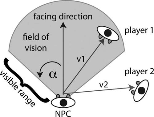
of treasure, the goal location is a moving player. The NPC detects the player within its field of vision using the vector between its position and the players. This is calculated as
direction = player.position - NPC.position;
The magnitude (length) of the direction vector represents the distance the player is from the NPC. If the angle between the facing vector and direction vector is less than the angle of vision and the magnitude of the direction vector is less than the visible range, then the player will be detected by the NPC.
The next workshop will demonstrate this in Unity.
![]() Unity Hands On
Unity Hands On
Line of Sight AI
Step 1. Download Chapter Five/ChasingAI.zip from the Web site. Open the chasingAI scene. In it you will find a large terrain and a solitary robot.
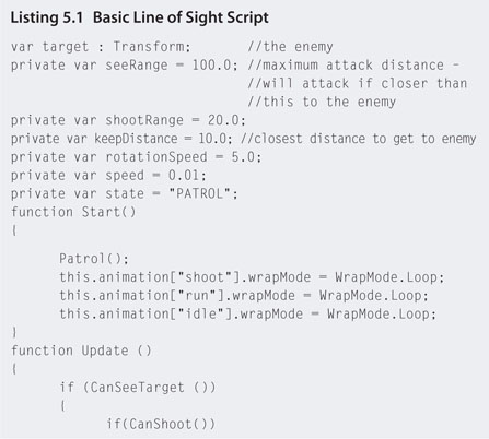
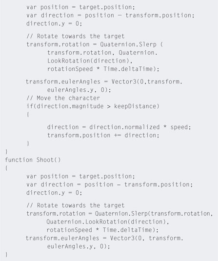
Step 2. Open the AI script with the script editor and add the code shown in Listing 5.1.

Step 3. Locate the AI script in the Inspector attached to the robot object in the Hierarchy. Drag and drop the First Person Controller from the Hierarchy onto the exposed target variable. This sets the object that the NPC will consider its enemy.
Step 4. Play. The CanSeeTarget() and CanShoot() functions use the variables seeRange and shootRange, respectively, to determine when the player is close enough to pursue and close enough to shoot. If you run away from the NPC backward as fast as possible you'll notice the point at which it gives up chasing you.
Step 5. The current code does not take into consideration the direction the NPC is facing. If you approach it from behind, it will still sense your presence when you are close enough. For it to use a field of vision angle, modify the AI script as shown in Listing 5.2.

Step 6. Play. You will now be able to sneak up behind the NPC without it noticing you.
5.3 Graph Theory
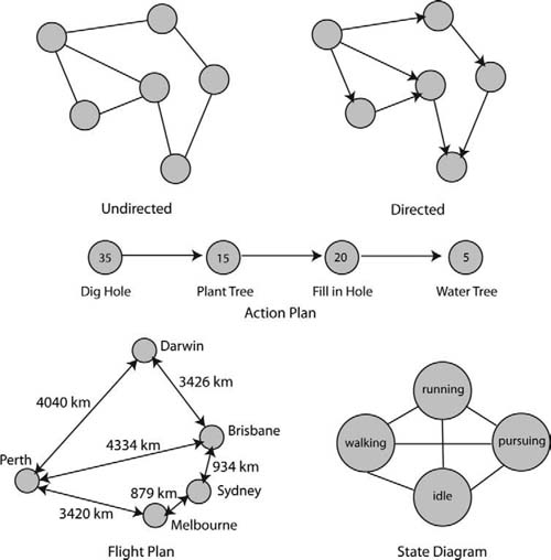
It would be impossible to begin talking about the ins and outs of AI without a brief background in graph theory. Almost all AI techniques used in games rely on the programmers having an understanding of graphs. A graph in this context refers to a collection of nodes and edges. Nodes are represented graphically as circles, and edges are the lines that connect them. A graph can be visualized as nodes representing locations and edges as paths connecting them. A graph can be undirected, which means that the paths between nodes can be traversed in both directions or directed, in which case the paths are one way. Think of this as the difference between two-way streets and one-way streets. Graphs are drawn with nodes represented as circles and edges as lines as shown in Figure 5.2. Nodes and edges can be drawn where nodes represent coordinates such as those on a flight plan or as symbolic states where the physical location in the graph is meaningless. For example, the state diagram in Figure 5.2 could be drawn with nodes in any position and any distance from one another. Some directed graphs allow bidirectional traversal from one node to another in the same way as undirected graphs. However, if arrows are already being used in a directed graph to show some one-way-only paths, they should also appear on bidirectional edges for consistency.
Both nodes and edges can have associated values. These values could be the distance between nodes, such as those representing distances in the flight plan of Figure 5.2, or the time it takes to complete an action, such as nodes in the action plan of Figure 5.2.
The ways in which graphs are useful in games AI will become evident as we progress through the chapter.
FIG 5.2 Undirected and directed graph representations and some examples.
5.4 Waypoints
The concept of waypoints was introduced in Chapter Four as a means of marking a route on a map that NPCs can follow. In the workshop we developed a very simple algorithm to cycle through the waypoints and have an NPC follow them continuously.
A waypoint is simply a remembered location on a map. Waypoints are placed in a circuit over the map's surface and are connected by straight line paths. Paths and waypoints are connected in such a way that an NPC moving along the paths is assured not to collide with any fixed obstacles. Waypoints and their connecting paths create a graph. Moving from waypoint to waypoint along a path requires an algorithm to search through and find all the nodes and how they are connected to each other. An example maze and a set of waypoints are illustrated as a graph in Figure 5.3. The graph does not necessarily need to reflect the physical layout of the maze when drawn. This example only shows which nodes connect to other nodes, not the location of the nodes or the distances between them.
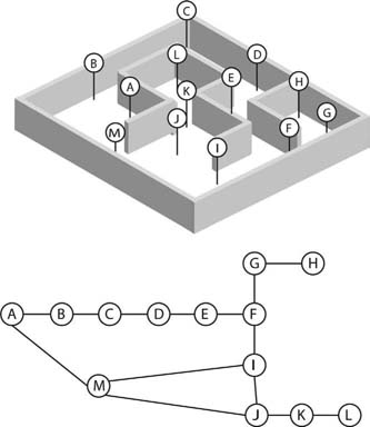
FIG 5.3 A maze with a set of waypoints.
In the graph of Figure 5.3, an NPC wanting to move from waypoint A to waypoint L could not simply plot a straight line between the two waypoints as they are not connected directly by an edge. The NPC then has the choice of navigating from waypoint A to waypoint L with the following sequences: A,M,J,K,L or A,B,C,D,E,F,I,J,K,L or A,M,I,J,K,L. The second sequence is obviously longer than the others, although all are legitimate paths. So how do you determine the best path from one waypoint to another?
Usually you will want an NPC to move from one waypoint to another via the shortest path. Often the meaning of shortest refers to the Euclidian distance between points, but not always. In real-time strategy (RTS) games where maps are divided up into grids of differing terrain, the shortest path from one point to another may not be based on the actual distance, but on the time taken to traverse each location; for example, the shortest Euclidean distance from point C2 to point A2 of Figure 5.4 will take an NPC through a river. Moving through the river may take the NPC twice as long as if it were to go the longer distance across the bridge. The definition of shortest is therefore left up to a matter of utility. The term utility originates in classical game theory and refers to the preferences of game players. If time is more important to an NPC than distance,

FIG 5.4 An example tiled strategy game map showing different terrain and a graph with utilities.
then the NPC will place a higher utility on time, thus avoiding the river. Utility values can be represented on a graph as weights on the edges, as shown in Figure 5.4. In this example, to travel from waypoint C2 to A2 directly via B2 will cost the NPC 3+3 = 6 points. Assuming a high number means less desirable, we might attribute these weights with travel time and say this route will take the NPC 6 hours. Further examination of the graph shows that it will only cost 4 hours to travel from waypoint C2 to A2 via points C1, B1, and A1.
In order to implement waypoints effectively in a game there needs to be an efficient way to search through them to find the most appropriate paths.
5.4.1 Searching Through Waypoints
There are High methods to find the shortest path from one node to another in a graph. These include algorithms such as breadth-first search (BFS) and depth-first search (DFS).
The BFS takes the given starting node and examines all adjacent nodes. Nodes that are adjacent to a starting node are ones that are connected directly to the starting node by an edge. In turn, from each of the adjacent nodes, nodes adjacent to these are examined. This process continues until the end node is found or the search for adjacent nodes has been exhausted. The algorithm can be written as Listing 5.3.

This algorithm will always find the shortest path (Euclidean distance) from the start to the end vertices, assuming that each vertex is the same distance apart. For example, in a maze game where the environment is represented by a grid of squares of equal size, each square represents a node for the purposes of the algorithm. As shown in Figure 5.5, the starting square is labeled with a 1. Radiating out from this square, all adjacent squares are labeled with a 2. All squares adjacent to the 2 squares not already labeled with a 1 or a 2 are labeled with a 3. This process continues until the destination square is found. This can be quite a long way of searching, as almost all squares in the grid will be examined. This algorithm can be
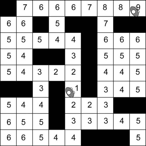
FIG 5.5 Environment map for a maze with path found using BFS.
modified to take into consideration other costs such as terrain type and traversal times in addition to or instead of distance by keeping track of all possible paths to the destination and adding up the costs. The path with the least cost can then be selected.
The DFS is simpler than the BFS and hence less effective. Instead of radiating out from the starting node, this algorithm simply follows one adjacent node to the next until it reaches the end of a path. Recursion works well for this algorithm and can be written as Listing 5.4.

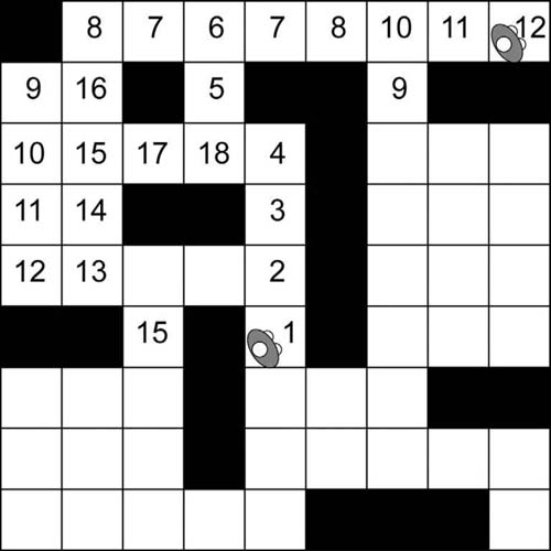
FIG 5.6 Environment map for a maze with path found using DFS.
An implementation of this algorithm is shown in Figure 5.6. Note that the algorithm does not find the shortest path to the destination, just a path. The success of finding the destination in a reasonable time is left to the luck of which adjacent node is selected first. In Figure 5.6, nodes are selected in an anticlockwise order beginning with the one immediately above the current node. If a clockwise order had been chosen the path would be different. Of course, this algorithm could also be modified to perform an exhaustive search to find all paths to the destination; by finding the path with a minimum cost the best could be selected. However, it is an ineffective way of finding the shortest path.
The most popular algorithm used in games, for searching graphs, is called A* (pronounced A-Star). What makes A* more efficient than BFS or DFS is that instead of picking the next adjacent node blindly, the algorithm looks for one that appears to be the most promising. From the starting node, the projected cost of all adjacent nodes is calculated, and the best node is chosen to be the next on the path. From this next node the same calculations occur again and the next best node is chosen. This algorithm ensures that all the best nodes are examined first. If one path of nodes does not work out, the algorithm can return to the next best in line and continue the search down a different path.
The algorithm determines the projected cost of taking paths based on the cost of getting to the next node and an estimate of getting from that node to the goal. The estimation is performed by a heuristic function. The term heuristic seems to be one of those funny words in AI that is difficult to define. Alan Newell first defined it in 1963 as a computation that performs the opposite function to that of an algorithm. A more useful definition of its meaning is given by Russell and Norvig in Artificial Intelligence published in 1995. They define a heuristic as any technique that can be used to improve the average performance of solving a problem that may not necessarily improve the worse performance. In the case of path finding, if the heuristic offers a perfect prediction, that is, it can calculate the cost from the current node to the destination accurately, then the best path will be found. However, in reality, the heuristic is very rarely perfect and can only offer an approximation.
![]() Unity Hands On
Unity Hands On
Pathfinding with A*
Step 1. Download Chapter Five/Waypoints.zip from the Web site. Open the project and the scene patrolling. Programming the A* algorithm is beyond the scope of this book and has therefore been provided with this project. If you are interested in the code, it can be found in the Project in the Plugins folder.
Step 2. Locate the robot model in the Robot Artwork > FBX folder in the Project. Drag the model into the Scene as shown in Figure 5.7. For the terrain and building models already in the scene, the robot will need to be scaled by 400 to match. If the textures are missing, find the material called robot-robot1, which is on the roothandle submesh of the robot; set it to Bumped Diffuse; and add the appropriate textures for Base and Normalmap. The texture files will be in the Project. The model may also have a cube on its head. Make this invisible by finding the headhandle subobject of the robot in the Hierarchy and unticking its Mesh Renderer.
Step 3. Waypoints can be added to the scene in the same way as they were in Chapter Three. Any GameObject can act as a waypoint. Create 9 spheres and arrange them in a circuit around the building. Add a 10th sphere out the front and an 11th sphere in the driveway as shown in Figure 5.8. Name the spheres Sphere1, Sphere2, etc.
Step 4. Create a new JavaScript file called patrol and open it in the script editor. Add the code shown in Listing 5.5.
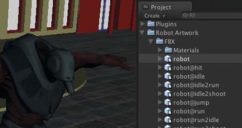
FIG 5.7 A robot model added to the scene and scaled by 400.

FIG 5.8 Waypoint layout.

Step 5. Attach the patrol script to the robot in the Hierarchy. Add the waypoints in order to the Waypoints array of the patrol script as shown in Figure 5.9.
Step 6. Play. While playing, switch to the Scene. The code in the Update function will draw lines along the edges. The blue tip indicates the
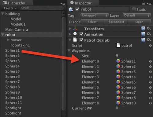
FIG 5.9 Adding waypoints to the patrol script.
direction of the path. If you have all the waypoints collected correctly, there should be a circuit around the building.
Step 7. To get the robot guard to patrol around the building, modify the patrol code as shown in Listing 5.6.
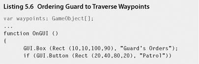
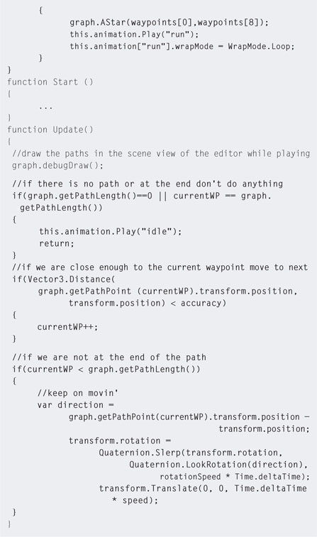
Step 8. Play. When the Patrol button is pressed the A* algorithm will calculate a path between the first and last waypoint and the guard will start running around it.
The character in this instance will move between the positions of waypoints. If you have placed your spheres on the ground, the character will sink into the ground as it is aiming its (0,0,0) position, which is in the center of the model, to the (0,0,0) of the sphere. To make the character appear to be moving on the terrain, move the spheres up to the right height. You can do this collectively by selecting all spheres in the Hierarchy by holding down shift while clicking on them and then dragging them up in the Scene.
In addition, if a character ever gets to a waypoint and starts circling it unexpectedly, it will be the accuracy setting. You may have it set to small; if the character can never get close enough to a waypoint it will just keep trying. In this case, set the accuracy value to something higher.
Step 9. Using the A* algorithm to calculate a circuit is a little bit of overkill, as a circuit can be performed simply using the code from Chapter Three. So now we will put it through its paces by adding some more button commands to get the character to move about the building. Modify the patrol code to that in Listing 5.7.
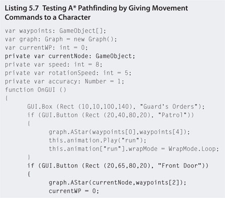
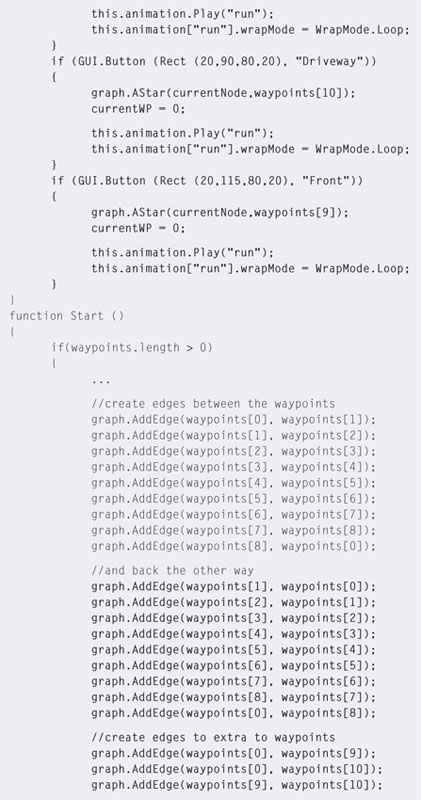

Step 10. The preceding code adds extra paths between the original circuit waypoints to point back the other way. This makes it possible to travel in any direction between points. Extra paths are also added between points in the driveway and out the front of the building. Play and switch to the Scene to see the red lines connecting the points (illustrated in Figure 5.10).
A new variable called currentNode has also been added to keep track of the waypoint the character last visited. This enables the algorithm to plot out paths based on the character's current position to the destination node.
This waypoint system is used in the next workshop after the development of a self-motivated character is explained.
5.5 Finite State Machines
The most popular form of AI in games and NPCs is nondeterministic automata, or what is more commonly known as finite state machines (FSM). An FSM can be represented by a directed graph (digraph) where the nodes symbolize states and the directed connecting edges correspond to state transitions. States

FIG 5.10 Debug lines showing paths in a waypoint graph.
represent an NPC's current behavior or state of mind. Formally, an FSM consists of a set of states, S, and a set of state transitions, T. For example, an FSM might be defined as S = {WANDER, ATTACK, PURSUE} and T={out of sight, sighted, out of range, in range, dead} as shown in Table 5.1.
In short, the state transitions define how to get from one state to another. For example, in Table 5.1, if the NPC is in state WANDER and it sights its opponent, then the state transitions to PURSUE. The state is used to determine elements of the NPC's behavior, for example, when the NPC is in state ATTACK the appropriate attacking animation should be used.
TABLE 5.1 State transition for an FSM |
|||||
| Transitions (opponent is…) | |||||
| State | out of sight | sighted | out of range | in range | dead |
| WANDER | WANDER | PURSUE | - | - | - |
| PURSUE | WANDER | - | PURSUE | ATTACK | - |
| ATTACK | - | - | PURSUE | ATTACK | WANDER |
Programming an FSM is a case of providing an NPC with a state value that represents its current behavior. Each state is accompanied by an event value representing the status of that state. The event tells us if the NPC has just entered that state, has been in the state for a while, or is exiting the state. Keeping track of this is critical for coordinating NPC movements around the environment and its animations. The FSM runs each game loop; therefore, knowing where the NPC is within a state is important for updating its status, the status of other game characters, and the environment.
For example, consider a Sim whose state changes to “take bath.” Before it can take a bath, it needs to make its way to the bathroom, run the bath, get undressed, and hop in the bath. This would happen on entering the state. The state would then enter update mode where the Sim is sitting in the bath washing itself, singing, blowing, bubbles, and so on. Once the Sim is clean, the state transitions to the exit phase in which it gets out of the bath and redresses. In pseudocode, the code might look something like that in Listing 5.8.

The FSM works by entering a state and then transitioning from enter, through update to exit. At the end of each event, the event is updated such that the next loop the FSM runs the code goes into the next event. On exiting a state, the state value is changed to something else and the event is set to enter.
![]() Unity Hands On
Unity Hands On
Implementing an FSM
In this workshop you will learn how to implement an FSM in conjunction with a waypoint system and the A* algorithm to program a guard character that patrols a warehouse and pursues intruders.
Step 1. Download Chapter Five/FSM.zip from the Web site and open the scene warehousePatrol. In the Scene you will see the warehouse model, the robot from the last workshop, and a waypoint system of spheres.
Step 2. Create a new tag named waypoint and set it for the tag of each sphere.
Step 3. Create a new JavaScript file called patrol and open with the script editor. Enter the code in Listing 5.9 and attach it to the robot.
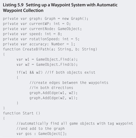
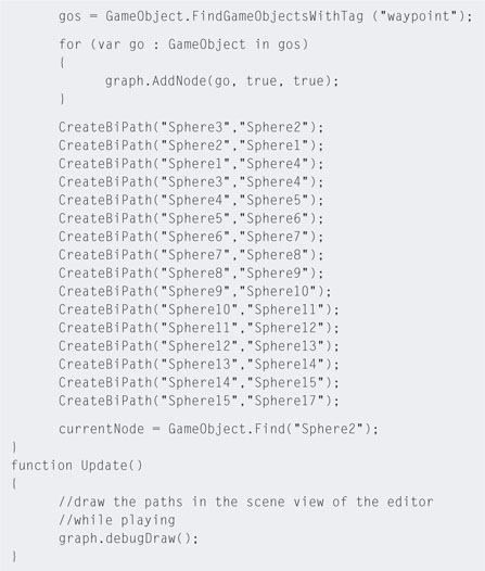
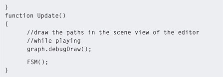
Step 4. Play. Go into the Scene view and have a look at the paths that have been created. In this code, a function has been written to help take away part of the laborious job of programming which points connect by creating bidirectional paths. This code also populates the waypoint graph automatically by looking for all the spheres that were tagged with waypoint in the Start() function.
Step 5. Locate Sphere2 and place the guard model near it as it has been set as the initial value for currentNode and will be used as the starting location of guard. Alternatively, you could add code such as this.transform.position = currentNode .transform.position to the end of the Start() function to have the code place the model.
Step 6. Modify the patrol script to that in Listing 5.10.
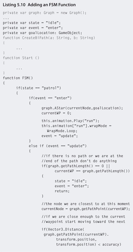
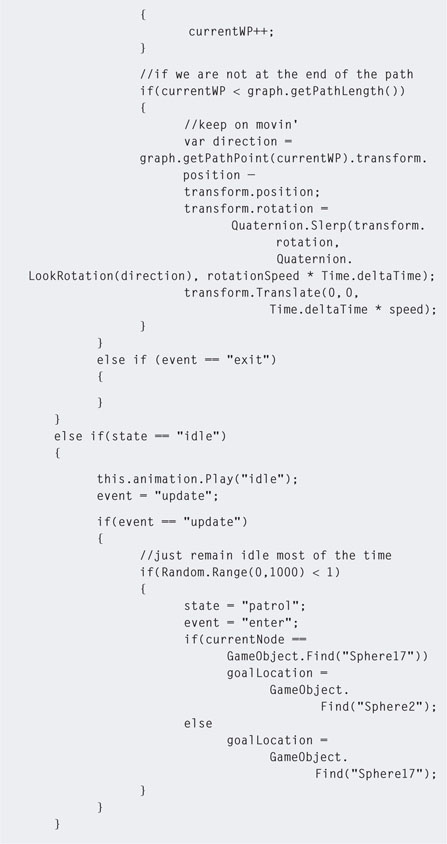
Step 7. Play. With the 1 in 1000 chance of the guard going into patrol mode, if you watch it for a while it will start moving from its current location to the last waypoint. When it gets there it will go into idle mode again, until after another 1 in 1000 chance it will start to patrol back in the other direction. Note that as with the waypoints in the previous workshop, the spheres may need to be moved up so that the guard model doesn't sink into the floor.
Step 8. Select Assets > Import Package > Character Controller from the main menu to add the First Person Controller prefab to the Project.
Step 9. Drag the First Person Controller prefab from the Project into the Hierarchy. Delete the existing main camera, as the First Person Controller has its own camera.
Step 10. Move the First Person Controller into the same room as the guard so you can watch it moving.
Step 11. In the Hierarchy, shift-select all the polySurface submeshes of the warehouse model and select Components > Physics > Mesh Collider to add colliders to the warehouse. Without the colliders, the First Person Controller will fall through the floor.
Step 12. Play. You will now be able to watch the guard patrolling from the first person view.
Step 13. The guard model will seem dark as there is no directional light so add one to the scene.
Step 14. Next we are going to add code to make the guard shoot and chase the player. To do this, add pursue and attack states as shown in Listing 5.11.


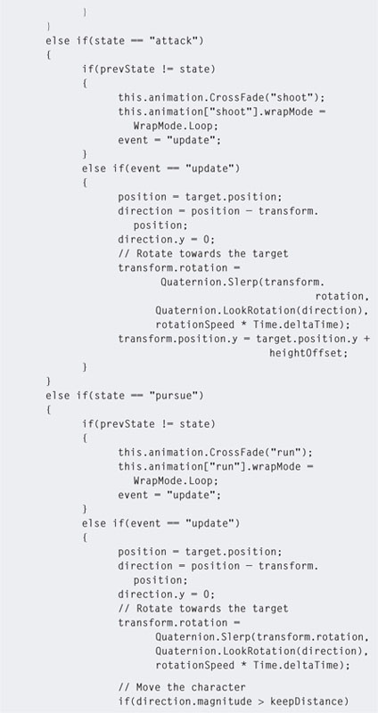

Step 15. The preceding code now controls the shooting and pursuing actions of the guard. Setting the state's event to enter has also been replaced. If the NPC's previous state was different from the current state, it runs the original event = “enter” code—the same as initializing a state. The distance the NPC shoots and pursues is controlled by variables at the
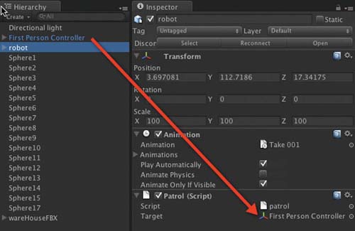
FIG 5.11 Setting the first person controller as the target for an NPC.
top of the code. Before playing, locate the patrol script attached to the robot model in the Hierarchy and set the target variable to the First Person Controller as shown in Figure 5.11.
When the NPC is pursuing and attacking the player, its position is made relative to the player. Because the model sizes of the player and the robot mesh are different sizes and the center points differ with respect to their y position, without some kind of height offset for the robot, it will either sink into the ground or float above it. This is the same issue the NPC has when following the waypoints and the reason why spheres are lifted above the ground. To fix this, the heightOffset variable has been added.
To get the best offset value usually the game needs to be played a number of times and the NPC observed. If you know the exact height of the model's mesh and its center position, it could be calculated.
Step 16. Play. The guard will chase and shoot at the player, but move up the stairs into another room and see what happens. The guard will follow the player but take shortcuts through the walls of the warehouse.
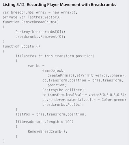
Step 17. This presents another problem to solve. We could make the NPC stick to the waypoints and paths while trying to follow the player, but what if the player goes somewhere there are no waypoints? You could also spend a lot of time placing waypoints all over the map as a solution. However, a simpler solution is to place temporary waypoints down on the map that draw out the path the player is walking and have the NPC follow them instead. This is another common technique used in games called breadcrumb pathfinding. To develop a simple breadcrumb script, create a new JavaScript file called breadcrumbs and add the code in Listing 5.12.
Step 18. Attach this script to the First Person Controller.
Step 19. Play. Walk backward and look at the green spheres being added to the map. These are your breadcrumbs. They mark the last 100 locations your First Person Controller was on the map. Of course, in a real game you wouldn't see these but they are added here for illustrative purposes.
Step 20. To get the NPC to follow these breadcrumbs when it is in pursuit, modify the patrol script as shown in Listing 5.13.
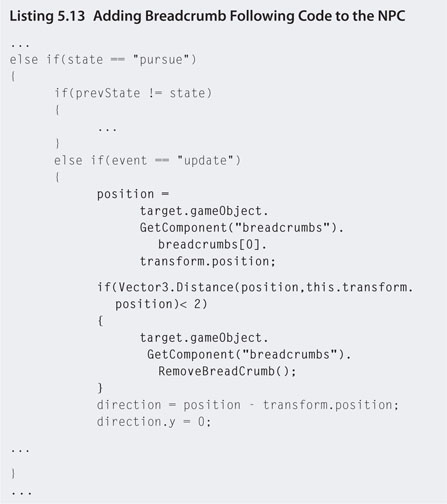
Step 21. Play. When the NPC is in pursuit of the player it will follow the breadcrumb trail. As it reaches a breadcrumb it deletes it from the player's breadcrumb array.
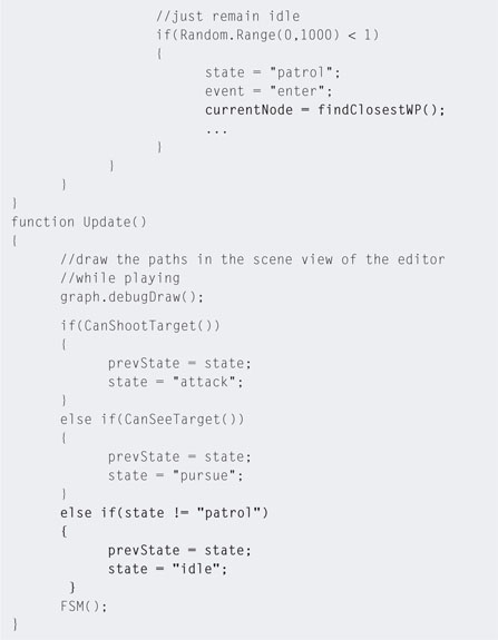
Step 22. Last but not least, we want the NPC to continue patrolling when the player manages to move beyond its range. To do this we need to set the state to idle and also find the NPC its closest waypoint. That way the A* algorithm can work to set the NPC back on its patrol path. To do this, modify the patrol script to that in Listing 5.14.


Step 23. Play. If you can manage to outrun the NPC, you will find that it goes into idle mode and then resumes its patrolling path.
5.6 Flocking
When you observe the movement of crowds or groups of animals their motions appear aligned and coordinated; for example, a flock of birds flying across the sky appears synchronized, staying together as a group, moving toward a common goal, and yet not all following the exact same path.
Applying flocking principles to NPCs in a game can add extra realism to the environment as secondary animations. If the game is set in a jungle setting, having a flock of birds fly across the sky looks far better than random birds flying in random directions.
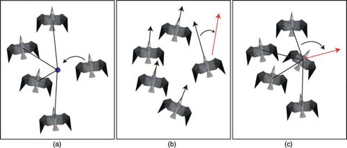
FIG 5.12 Flocking rules: (a) move toward average group position, (b) align heading with average group heading, and (c) avoid others.
In 1986, Craig Reynolds developed an unparalleled simple algorithm for producing flocking behavior in groups of computer characters. Through the application of three rules, Reynolds developed coordinated motions such as that seen in flocks of birds and schools of fish. The rules are applied to each individual character in a group with the result of very convincing flocking behavior. These rules (illustrated in Figure 5.12) include
- moving toward the average position of the group
- aligning with the average heading of the group
- avoid crowding other group members
Flocking creates a moving group with no actual leader. The rules can be increased to take into consideration moving toward a goal position or the effect of wind. These rules are used to create a flock of birds in the following workshop.
![]() Unity Hands On
Unity Hands On
Flocking
Step 1. Download Chapter Five/flocking.zip from the Web site and open the testFlock scene. Play. You will see a radar showing the position of seagulls created with the globalFlock script attached to the camera. To move the camera, use the arrow keys. This will allow you to look at parts of the flock. Currently the seagulls do not move. In the globalFlock script 100 seagulls are being created. If you want more, change the value of 100. If your computer starts to slow you may need to reduce the flock size.
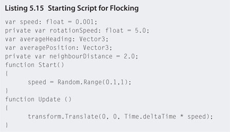
Step 2. Open the flock script and add the code in Listing 5.15.
Step 3. Attach the flock script to the SeagullPrefab in the Project.
Step 4. Play. Each seagull will have a random speed setting and be flying in a straight line. You can use the arrow keys to follow the birds.
Step 5. Let's apply the first flocking rule to the population. Modify the flock script as shown in Listing 5.16.


Step 6. Play. Small flocks will form in the population. In the script, Random.Range is used to apply the rules about one in five game loops. This ensures that not all the birds have the rules that run each game loop. If this happens, the application runs very slowly and gets slower the more birds you have. Note that the average position is also only determined for neighboring birds, not the whole population. This is determined by the neighbourDistance variable. If you make this value larger, you will get one big flock.
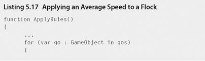
Step 7. Currently, because the birds have random speeds, birds will eventually break away from their flocks because they can't keep up or are going too fast. To keep them together, the second rule is applied. Birds in the flock match the average speed. To achieve this, modify the flock script to that in Listing 5.17.

Step 8. Play. Averaging of the speed will help keep the formed flocks together.
Step 9. Finally, adding the third rule will enable the birds to keep out of each other's way. Before changing the code, observe the current flocking movement. Once a bird is flying in a circular pattern within the flock it stays with that pattern. Now change the flock script to that in Listing 5.18.
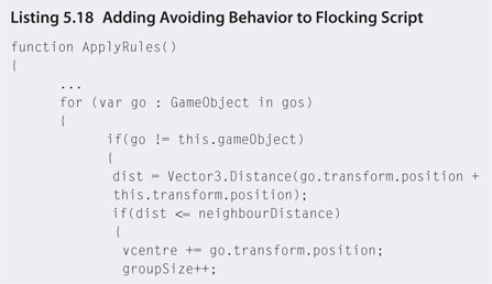
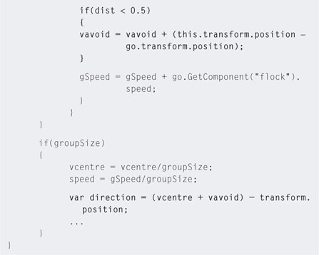
Step 10. Play. Take a close look at the birds' behavior. You will notice they now dart out of the way in a similar movement to what is observed in real flocking birds.
So far, the flocks created are reminiscent of crows or vultures circling in the sky around their next meal. This could be used for a dramatic effect in a game to point out the position of something sinister in the game environment. More often than not, flocks used for ambience tend to be traveling across the scene. To achieve this type of flocking, more rules can be added.
Step 11. To make the birds move across an endless sky, we can add a wind value. This is a vector indicating the direction of travel. Modify the flock script to that in Listing 5.19.


Step 12. Play. The added wind vector will cause the birds to fly along the same course. The birds will still flock together, but instead of circling they will form close-streamed groups.
Step 13. If you want the birds to fly across the screen to a particular location, a goal position can also be added to the rules. Modify the flock script to that in Listing 5.20.
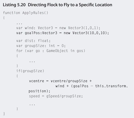
Step 14. Play. The birds will form into groups flying toward a single goal location.
These very flocking rules have been used in movies to create flocking characters. They were used in Batman Returns to create realistic swarms of bats and in The Lion King for a herd of wildebeest.
The rules can also be modified in games to develop intelligent group enemy behavior and optimize processing speeds. For example, in the workshop that introduced breadcrumb path finding, if there were hundreds of enemies, having them all process the breadcrumbs could prove computationally costly. Furthermore, if each one even had to run the A* algorithm, it could certainly slow down performance. However, if just one leader followed the breadcrumbs, the rest could flock and follow that leader.
5.7 Decision Trees
Decision trees are a hierarchical graph that structure complex Boolean functions and use them to reason about situations. A decision tree is constructed from a set of properties that describe the situation being reasoned about. Each node in the tree represents a single Boolean decision along a path of decision that leads to the terminal or leaf nodes of the tree.
A decision tree is constructed from a list of previously made decisions. These could be from experts, other players, or AI game experience. They are used in Black & White to determine the behavior of the creature. For example, a decision tree based on how tasty the creature finds an object determines what it will eat. How tasty it finds an object is gathered from past experience where the creature was made to eat an object by the player.
To illustrate the creation of a decision tree for an NPC, we will examine some sample data on decisions made about eating certain items in the environment. The decision we want made is a yes or no about eating given the characteristics or attributes about the eating situation. Table 5.2 displays some past eating examples.
Given the attributes of a situation (hungry, food, and taste), a decision tree can be built that reflects whether the food in question should be eaten. As you can see from aforementioned data, it is not easy to construct a Boolean expression to make a decision about eating. For example, sometimes it does matter if the NPC is hungry and other times it does not; sometimes it matters if the food is tasty and sometimes it does not.
To construct a decision tree from some given data, each attribute must be examined to determine which one is the most influential. To do this, we examine which attributes split the final decision most evenly. Table 5.3 is a count of the influences of the given attributes.
TABLE 5.2 Examples for making an eating decisiona |
||||
| Example | Attributes | Eat? | ||
| Hungry | Food | Taste | ||
| 1 | Yes | Rock | 0 | No |
| 2 | Yes | Grass | 0 | Yes |
| 3 | Yes | Tree | 2 | Yes |
| 4 | Yes | Cow | 2 | Yes |
| 5 | No | Cow | 2 | Yes |
| 6 | No | Grass | 2 | Yes |
| 7 | No | Rock | 1 | No |
| 8 | No | Tree | 0 | No |
| 9 | Yes | Tree | 0 | Yes |
| 10 | Yes | Grass | 1 | Yes |
aValues for the attribute taste are 0 for awful, 1 for ok, and 2 for tasty. |
||||
TABLE 5.3 Attribute influence over the final eat decision |
||||
| Attribute | Eat = yes | Eat = no | Total influences |
|
| Hungry | ||||
| Yes | 5 | 1 | ||
| No | 2 | 2 | ||
| Total exclusive 0s | 0 | 0 | 0 | |
| Food | ||||
| Rock | 0 | 2 | ||
| Grass | 3 | 0 | ||
| Tree | 2 | 1 | ||
| Cow | 2 | 0 | ||
| Total exclusive 0s | 1 | 2 | 3 | |
| Taste | ||||
| 0 | 2 | 2 | ||
| 1 | 1 | 1 | ||
| 2 | 4 | 0 | ||
| Total exclusive 0s | 0 | 1 | 1 | |
To decide which attribute splits the eat decision, we look for examples where an attribute's value definitively determines if Eat is yes or no. In this case, when Food equals Rock, every instance of Eat is no. This means that we could confidently write a Boolean expression such as
if food = rock
then eat = no
without having to consider any of the other attributes. The total number of exclusive 0s counted in a column determines the attribute with the best split. By exclusive we mean that the value of the attribute must be 0 in one column and greater than 0 in another. If both columns were 0, then the value would have no effect at all over the decision. In the cases of Rock, Grass, and Cow, the final value for Eat is already known and thus these values can be used to create instant leaf nodes off the root node as shown in Figure 5.13. However, in the case of Tree, the decision is unclear, as sometimes Eat is yes and sometimes it is no.
To find the next best splitting attribute, outcome decisions involving the Tree value are combined with the remaining attributes to give the values shown in Table 5.4.
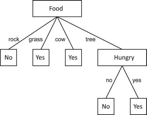
In this case, the second best attribute is Hungry. Hungry can now be added to the decision tree under the Tree node to give the graph shown in Figure 5.14. Note that the yes and no choices for Hungry provide definitive answers for Eat, and therefore the nodes do not need to be classified further with any other attributes. The decision tree in Figure 5.14 is the complete decision tree for data from Table 5.2. You could say in this case that the taste of the food is irrelevant.
FIG 5.13 Partial decision tree for data from Table 5.3.

FIG 5.14 Complete decision tree for eating objects.
A famous algorithm used for creating decision trees from examples (and that used in Black & White) is ID3 developed by computer scientist J.R. Quinlan in 1979.
![]() Unity Hands On
Unity Hands On
Decision Trees
In this workshop we create a very simple decision tree for an RTS AI game opponent that will decide on its strategy based on the map layout. The decision being made is about whether or not to give priority to mining for minerals and gas instead of building defenses or attacking the enemy. Based on the amounts of nearby minerals and gases, the ease of entry by which the enemy can access the base, and the overall distance to the enemy, a table with all combinations of the values for each decision variable (the attributes) is drawn up. Data for decision making are shown in Table 5.5.
In this case, data are fictitious; however, they could be gathered from other human players or experience from previous games.
TABLE 5.5 Data for RTS AI build decisions |
|||||
| Rule | Number of mineral resources nearby | Number of gas resources | Easy enemy access to base | Distance to enemy | Give priority to mining |
| 1 | Low | High | No | Far | Yes |
| 4 | Low | High | Yes | Far | Yes |
| 7 | Low | Low | No | Far | No |
| 10 | Low | Low | Yes | Far | No |
| 13 | High | High | No | Far | Yes |
| 16 | High | High | Yes | Far | Yes |
| 19 | High | Low | No | Far | Yes |
| 22 | High | Low | Yes | Far | Yes |
| 25 | Low | High | No | Close | Yes |
| 28 | Low | High | Yes | Close | No |
| 31 | Low | Low | No | Close | No |
| 34 | Low | Low | Yes | Close | No |
| 37 | High | High | No | Close | Yes |
| 40 | High | High | Yes | Close | Yes |
| 43 | High | Low | No | Close | Yes |
| 46 | High | Low | Yes | Close | No |
Step 1. Download Chapter Five/DecisionTrees.zip from the Web site and open the decisionTree scene in Unity. Play to see the decision tree constructed from data in Table 5.5. This tree is illustrated in Figure 5.15.

FIG 5.15 A tree graph produced from data in Table 5.5.
Note that the full code for decision tree construction using the ID3 algorithm is contained in the Plugins > ID3.cs file in the Project. The original code can be found at http://codeproject.com/KB/recipes/id3.aspx. Data have been changed to reflect the values in Table 5.5. Although we are not focusing on C# in this book, the complexities of most AI algorithms lend themselves to being written in more robust language than JavaScript. The objective here is not to teach you C# but rather to point out parts of the code you could experiment with changing should you want to create your own decision tree.
Step 2. Open ID3.cs in the script editor. Scroll to the very bottom of the code to find the createDataTable() function.
Step 3. First the attributes are defined. For each of these are a set of values. Data are then laid out in a table. The name of each column is the attribute name followed by a final decision column, in this case named strategy. Following this, each row from data is added to the table. If you want to create your own decision tree you can add as many attribute columns as you wish by following the same coding format. Just ensure that there is an associated column for each item in data. The last column, denoting a decision, is a Boolean value.
Decision trees provide a simple and compact representation of complex Boolean functions. Once constructed, a decision tree can also be decomposed into a set of rules. The beauty of the decision tree is that the Boolean functions are learned from a set of complex data that could take some time for a programmer to deconstruct manually into rules. In addition, a decision tree can be updated as the program runs to incorporate newly learned information that may enhance the NPC's behavior.
5.8 Fuzzy Logic
Fuzzy logic provides a way to make a decision based on vague, ambiguous, inaccurate, and incomplete information. For example, properties such as temperature, height, and speed are often described with terms such as too hot, very tall, or really slow, respectively. On a daily basis we use these terms to make decisions with the unspoken agreement as to the interpretation of such vague statements. If you order a hot coffee, for example, you and the barista have an idea for a range of temperatures that are considered hot (for coffee).
Computers, however, only understand exact values. When you set the temperature on an oven to cook a pie you give it an exact temperature—you can't tell it you want the pie just hot. There is, however, a type of computational logic system that interprets vague terminology by managing the underlying exactness of the computer. It is called fuzzy logic. It is based on the concept that properties can be described on a sliding scale.
Fuzzy logic works by applying the theory of sets to describe the range of values that exist in vague terminologies. Classical set theory from mathematics provides a way of specifying whether some entity is a member of a set or not. For example, given the temperatures a = 36 and b = 34 and the set called Hot, which includes all numerical values greater than 35, we could say that a is a member of the set Hot and b is not.
Classical set theory draws lines between categories to produce distinct true and false answers; for example, b = Hot would equate to false. Fuzzy logic blurs the borderlines between sets (or makes them fuzzy!). Instead of a value being a member of a set, fuzzy set theory allows for a degree of membership.
To illustrate this, Figure 5.16 conceptualizes the difference between classical and fuzzy sets—the difference being that values in fuzzy sets overlap. In this example, the lower ranges of warm values are also members of the cold set. Values in fuzzy sets are given a degree of membership value that allows them to be partially in one set and partially in another. For example, the temperature value 34 could be 20% in the cold set and 80% in the warm set.

FIG 5.16 Classical sets have distinct boundaries. Fuzzy sets do not.
A fuzzy rule can be written as
if x is A
then y is B
where x and y, known as linguistic variables, represent the characteristics being measured (temperature, speed, height, etc.) and A and B, known as linguistic values, are the fuzzy categories (hot, fast, tall, etc.). A fuzzy rule can also include AND and OR statements similar to those in Boolean algebra. The following are examples of fuzzy rules:
| if | temperature is hot | |
| or | UV_index is high | |
| then | sunburn is likely | |
| if | temperature is warm | |
| and | humidity is low | |
| then | drying_time will be quick |
Given a set of fuzzy rules and a number of inputs, an output value can be deduced using fuzzy inferencing. There are two common ways to inference on fuzzy rules: Mamdani style and Sugeno style, both named after their creators. The Mamdani style is widely accepted for capturing human knowledge and uses a more intuitive form of expressing rules.
The Mamdani style consists of four steps: fuzzification, rule evaluation, aggregation, and defuzzification. Consider the following rules by which an NPC may operate:
| Rule 1: | if | health is good | |
| and | shield is adequate | ||
| then | mood is happy | ||
| Rule 2: | if | health is bad | |
| or | shield is moderate | ||
| then | mood is indifferent | ||
| Rule 3: | if | health is bad | |
| and | shield is inadequate | ||
| then | mood is angry |
Fuzzification takes inputs in the form of discrete values for the NPC's health and shield strength and fuzzifies them. To fuzzify them, we simply pass them through the respective fuzzy sets and obtain their degrees of membership.
Rule evaluation involves substituting the degrees of membership into the rules given. For example, if the value for health is good was 17% and the value for shield is adequate was 25%, Rule 1 would become:
if 17% and 25% then mood is (17%) happy
Only the part of the rule in the if statement (shown in bold) has the fuzzy values substituted. If the values are connected by an AND, the smallest degree of membership is assigned to the then part. If the values are connected by an OR, the larger degree of membership is assigned. Assuming health is bad is 50% and shield is moderate is 25%, Rule 2 would become:
if 50% or 25% then mood is (50%) indifferent
These values are then used to clip the fuzzy sets for happy and indifferent pertaining to mood. In brief, 17% of the happy set and 50% of the indifferent set are merged to create a new fuzzy set as shown in Figure 5.17. This is the third step of Rule Aggregation.
The final step is defuzzification. This takes the final aggregated fuzzy set and converts it into a single value that will be the fuzzy output. The final fuzzy set contains the value; all that is needed is to extract it. The simplest method for doing this is called the centroid technique, which finds the mathematical center of gravity of the set. This involves multiplying all the values in the set with their degree of membership, adding them together, and dividing by the sum of all the degrees of membership in the set. This gives a percentage value, in this case, pertaining to the mood value. For example, the result might be a 40% mood that would result in the mood being indifferent.
Developing a fuzzy logic engine requires a great deal of understanding in programming and mathematics. There is certainly not enough room in this chapter to provide a full example. Therefore, the next workshop uses an Open Source fuzzy logic engine called DotFuzzy (available from http://havana7.com/dotfuzzy/) written in C#.
FIG 5.17 Merged fuzzy sets.

Fuzzy Logic
This hands-on session uses the DotFuzzy engine to create behavior rules for an NPC. The NPC's health and shield strength will be used to calculate its mood. Depending on its mood, it will decide to chase, attack, or ignore the player who is able to shoot at it.
Step 1. Download Chapter Five/FuzzyLogic.zip from the Web site and open the fuzzyAI scene. Play. You can walk around the scene and shoot spheres from the large gun being held by the player. In the middle of the environment you will find a robot. This robot has similar code to that used in the Line of Sight workshop; however, it will not attack you. The robot's health and shield strengths are displayed on the screen. If you shoot at the robot with the left mouse button, its health and shield strength will go down. If you leave the robot alone, it will recover after some time.
The DotFuzzy engine has been loaded and is in the Project Plugins folder.
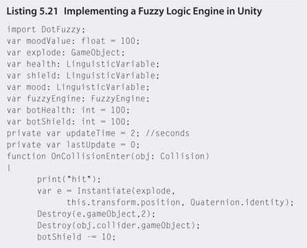
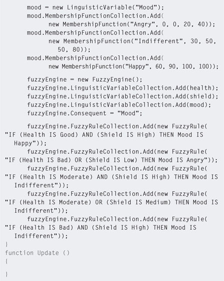
Step 2. Open the fuzzyBrain JavaScript file with the script editor. The linguistic variables for the engine are defined at the top. Add the code as shown in Listing 5.21.

![]() Note
Note
Defining Fuzzy Sets
Fuzzy sets are defined by four values representing the degrees of membership of values at each quarter. These four values can be seen in the MembershipFunction()s of Listing 5.21. Sets are drawn from four values given such that each value represents the x coordinate on a quadrilateral and the respective y values are 0, 100, 100, 0. The x values will vary among sets, but the y values are always the same. Figure 5.18 illustrates the sets associated with the linguistic variable Health.
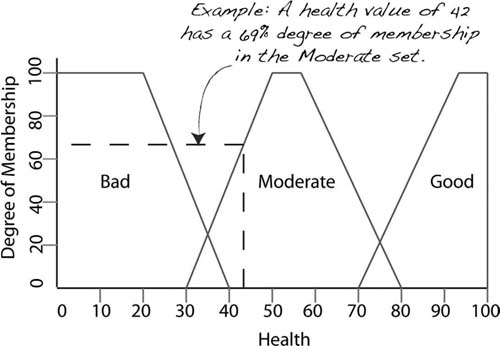
FIG 5.18 Visualizing a fuzzy set.
Step 3. Note in fuzzyBrain.js how the fuzzy rules are written out in an English-type manner. This allows you to write out your own fuzzy rules to suit the purposes of your NPC. Using fuzzy rules creates NPCs that are less predictable, as not even the programmer can be sure what they will do under specific conditions.
Step 4. Play. When you shoot at the robot, it will ignore you until its health and shield strength become reasonably low. When it is almost dead it will run away and wait for its strength to return. The robot model doesn't have a death animation and therefore when its health and shield reach 0 they stay at zero. You will not be able to kill it.
This workshop has provided a very brief overview of including fuzzy logic in a game environment. It demonstrates how to link the DotFuzzy engine into Unity. From this point you will be able to create your own rules and define fuzzy behaviors for other NPCs.
5.9 Genetic Algorithms
Evolutionary computing examines intelligence through environmental adaptation and survival. It attempts to simulate the process of natural evolution by implementing concepts such as selection, reproduction, and mutation. In short, it endeavors to replicate the genetic process involved in biological evolution computationally.
Genetics, or the study of heredity, concentrates on the transmission of traits from parents to offspring. It not only examines how physical characteristics such as hair and eye color are passed to the next generation, but it also observes the transmission of behavioral traits such as temperament and intelligence. All cells in all living beings, with the exception of some viruses, store these traits in chromosomes. Chromosomes are strands of deoxyribonucleic acid (DNA) molecules present in the nuclei of the cells. A chromosome is divided up into a number of subparts called genes. Genes are encoded with specific traits such as hair color, height, and intellect. Each specific gene (such as that for blood type) is located in the same location on associated chromosomes in other beings of the same species. Small variations in a gene are called alleles. An allele will flavor a gene to create a slight variation of a specific characteristic. A gene that specifies the blood group A in different people may present as an allele for A+ and in another person an allele for A-. Chromosomes come in pairs, and each cell in the human body contains 23 of these pairs (46 chromosomes total) with the exception of sperm and ova, which only contain half as much. The first 22 pairs of human chromosomes are the same for both males and females, and the 23rd pair determines a person's sex. At conception, when a sperm and ova meet, each containing half of its parent's chromosomes, a new organism is created. The meeting chromosomes merge to create new pairs. There are 8,388,608 possible recombinations of the 23 pairs of chromosomes with 70,368,744,000,000 gene combinations.
Evolutionary computing simulates the combining of chromosomes through reproduction to produce offspring. Each gene in a digital chromosome represents a binary value or basic functional process. A population is created with anywhere between 100 and many thousands of individual organisms where each individual is represented usually by a single chromosome. The number of genes in the organism will depend on its application. The population is put through its paces in a testing environment in which the organism must perform. At the end of the test each organism is evaluated on how well it performed. The level of performance is measured by a fitness test. This test might be based on how fast the organism completed a certain task, how many weapons it has accumulated, or how many human players it has defeated in a game. The test can be whatever the programmer deems is a best judgment of a fit organism. Once the test is complete, the failures get killed off and the best organisms remain.
These organisms are then bred to create new organisms, which make up a new second-generation population. Once breeding is complete, first-generation organisms are discarded and the new generation is put through its paces before being tested and bred. The process continues until an optimal population has been bred.
A chromosome in a genetic algorithm is represented by a string of numbers. Each chromosome is divided into a number of genes made up of one or more of the numbers. The numbers are usually binary; however, they need not be restricted to such.
Steps involved in a genetic algorithm are:
Create a population and determine the fitness
A genetic algorithm begins by specifying the length of a chromosome and the size of the population. A 4-bit chromosome would look like 1100. Each individual in the population is given a random 4-bit sequence. The population is then allocated some task. How each individual performs determines its fitness. For example, if the task is to walk away from a starting location, then individuals who walk the farthest are the fittest.
Mate the fittest individuals
The population is sorted according to fitness and the top proportions of the group are mated. This involves crossing their chromosomes to create new individuals. The process of crossover involves slicing the chromosomes and mixing and matching. For example, parents with chromosomes 0011 and 1100 with their chromosomes sliced half-way will produce offspring with chromosomes 0000 and 1111.
In nature, a rare event occurs in breeding called mutation. Here, an apparently random gene change occurs. This may lead to improved fitness or, unfortunately, a dramatically handicapped offspring. In evolutionary computing, mutation can reintroduce possibly advantageous gene sequences that may have been lost through population culling. Introducing new randomly generated chromosomes into the population or taking new offspring and flipping a gene or two randomly can achieve mutation. For example, an individual with a chromosome 0101 could be mutated by flipping the third gene. This would result in 0111.
Introducing the new population
The final step is to introduce the new population to the task at hand. Before this occurs, the previous population is killed off. Once the new population's fitness has been determined, they are again sorted and mated.
The process is a cycle that continues creating and testing new populations until the fitness values converge at an optimal value. You can tell when this has occurred as there will be very little change in the fitness values from population to population.
An example of a working genetic algorithm can be found in the Unity project available from the Web site as a download from Chapter Five/GeneticAlgorithms.zip. In this project, NPCs are programmed to navigate a maze based on genetic algorithms. Each generation has 60 seconds to explore as much of the maze as possible. The ones that explore the most are bred for the next generation.
Each NPC does not know what the maze looks like. It only has information on its current surrounding area. This information is coded into a binary sequence. From the NPC's location what is to the left, front, and right of it are recorded. Take, for example, the layout in Figure 5.19. To the left is a wall, to the front is a wall, and to the right is free space. This is coded with a 1 for a wall and a 0 for a space. In this example, the code would be 110 (wall to left, wall in front, and space to right).

FIG 5.19 An example maze layout.
The NPC has four actions available to it: move forward, turn left and move forward, turn right and move forward, and turn around and move forward. These are coded into the NPC's chromosome as 1, 2, 3, and 4 for each action, respectively.
Returning to the maze layout, at any position the NPC could be faced with one of six layouts. These being:
- [0,0,0], no walls
- [0,0,1], a wall to the right
- [0,1,1], walls to the front and right
- [1,1,1], walls left, front, and right
- [1,0,0], a wall to the left
- [1,0,1], walls to the left and right
For each possible maze configuration, the NPC has an associated action. In this case, the NPC's DNA is six chromosomes long. An example is shown in Figure 5.20.
In Figure 5.20, if the NPC encounters a wall to the right only, its associated action is 2, meaning turn left and move forward. In the case of a wall to the

FIG 5.20 All possible maze configurations and an example NPC DNA string.
front and right, the action tells the NPC to move forward. This is obviously a bad choice, but nonetheless, the NPC has nothing to go on but the actions provided in its DNA. The fewer times an NPC's DNA leads it into a wall, the farther it will get exploring the maze.
In the beginning, 100 NPCs are created each with random DNA setting. The NPCs are allowed to explore the maze. The ones that get the farthest will have DNA sequences that allow them to move farther. These are the ones kept for breeding. Now and then mutations are thrown in to create DNA sequences that may not occur from the natural selection process. Results from 10 generations of this program are shown in Figure 5.21. Feel free to download the code and play around with it for yourself.
5.10 Cellular Automata
Many strategy and simulation games are played out on a grid. The best example is SimCity. The AI running beneath SimCity is a cellular automata. In short, a cellular automata is a grid of cells with associated values where each value is updated constantly by the value in neighboring cells. SimCity uses this mechanism to decide what happens in associated cells based on what the player is doing. For example, if the player puts a nuclear power plant in a particular location, any mansions in surrounding cells become worthless and soon the occupants will move out. Cells between an apartment block and the bus stop will affect the distance the occupants must travel to work and also the occupancy rate. Such a simple AI mechanic can create some very complex-looking relationships.
One of the most famous cellular automata is the Game of Life developed by researcher John Conway in 1970. It is an infinite 2D grid of cells. Each cell can be in one of two states: dead or alive. The state of the cell is based on

FIG 5.21 A maze exploring genetic algorithms over 10 generations.
the states of its closest eight neighbors. Each update, the status of the cell is calculated using four rules. These are:
- If the cell is alive but has less than two alive neighbors, it dies
- If the cell is alive and has two or three alive neighbors, it remains alive
- If the cell is alive but has more than three alive neighbors, it dies
- If the cell is dead but has exactly three alive neighbors, it becomes alive
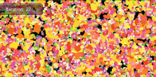
In the same way that the simple flocking rules create complex behaviors, so too does the Game of Life. An example run of the Game of Life is shown in

FIG 5.22 The Game of Life.
Figure 5.22. The Unity project for this can be downloaded from Chapter Five/CellularAutomata.zip.
5.11 Summary
This chapter has given a broad but brief introduction to some of the AI techniques used in games. There are numerous other AI techniques, such as neural networks and Bayesian networks, that have not been covered. Many of the topics are complex mathematically; if you require a deeper understanding of the domain, there are many good books available dedicated to the topic.
If you are interested in checking out some more uses of AI in games, the author highly recommends these Web sites:
for now though, it is hoped that you've come to appreciate the beauty of AI in the examples contained herein and opened up a new realm of possibilities for implementation of these mechanics in your own games.