6.1.1. Squeezing Flow of a Newtonian Fluid

The approach is based on two flat, circular discs with the radius R and a Newtonian fluid with the viscosity η in between. The gap between the two discs is 2h⁰. To the circular disks, a force of F is applied (Fig. 6.1).

Figure 6.1. A Newtonian fluid with the viscosity η is compressed by the force F acting on circular discs.

The force F exerts a pressure on the fluid, which induces compressive stresses in the fluid. These stresses cause a radial flow of the fluid from the disc center outwards to its circumference. The flow is based on a pressure difference dp. Under the influence of the force dF, the gap between the two discs is decreased by dh. The volume flow leaving the gap between the discs has to be equal to the displaced volume per time unit caused by the motion of the two discs.

(6.1)

Because of a decreasing gap and an increasing displaced volume, the required force to maintain a constant motion of the disc will increase significantly. The equation to describe this behavior can be deduced under the following boundary conditions.

• The problem will treated as a steady-state hydrodynamic problem.
• The radial velocity of the fluid is a function of the radius r and the vertical distance of both plates z: ν^r = ν^r(r, z).
• The vertical velocity of the fluid depends only on the distance: ν^z = ν^z(z).
• The pressure p is a function of the radius: p = p(r).
• The ambient pressure is p^a.

First the equations of change have to be defined:(6.2)

(6.3)

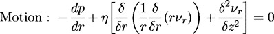
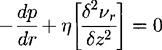
Because of the postulate that v^z does not depend on r and has a form like v^r = rf(z), the equation for the motion can be described as

(6.4)

The integration of the equation of continuity over z = 0 to z = h, and over the radius from r = 0 to r = r, results in

(6.5)with(6.6)

The integration of the equation of the motion with respect to z under the following boundary conditions f = 0 at z = h and f′(z) = 0 at z = 0 results in

(6.7)

Substitution of Equation 6.7 into Equation 6.5 results in

(6.8)

The combination of Equations 6.7 and 6.5 results in an equation describing the radial velocity of the fluid in terms of the motion of the plates, .

(6.9)

The integration of Equation 6.8 results in an equation for the radial pressure distribution:(6.10)

The calculation of the required force F(t) to be applied in order to maintain the disc motion h(t) requires first the calculation of the shear stress distribution τ^zz over the height h.

(6.11)

With this equation for the shear stress, the required force for a constant motion of the plates is calculated to:(6.12)

Equation 6.12 is called the Stefan equation [1] and describes the required force for a constant molding velocity. In the case of a constant force, Equation 6.12 has to be solved for h(t) and results in:(6.13)

Equation 6.13 describes the distance of both plates under a constant force of the elapsed time t.

Referring to an initial thickness of h⁰ = 1, Equation 6.13 can describe the achievable thickness of a residual layer under a constant molding force:(6.14)

This equation can be transferred to the hot embossing process with regard to molding force, molding velocity, and thickness of the residual layer. Therefore, fundamental relationships of molding can be derived. Otto et al. [30] developed, on the basis of squeeze flow, an equation for the residual thickness under the consideration of elevated and recessed structures. Bogdanski et al. [5] modified the equation of squeeze flow for a number of periodically arranged cavities with defined width and height. Independent of the modifications, the fundamental relationships can be described.

6.1.1.1. Velocity-Controlled Molding

• For the molding step of velocity-controlled molding, the molding force is proportional to the fourth power of the radius.(6.15)
• The molding force is proportional to the reciprocal value of the third power of the thickness of the achievable residual layer.(6.16)
• The molding force is only linearly proportional to the molding velocity and the viscosity of the (Newtonian) fluid.(6.17)(6.18)

These fundamentals have to be taken into account, for example, when the molding area increases. On the one hand, to obtain the same thickness of the residual layer for an area 2 times larger, a molding force 16 times higher is needed. On the other hand, if the thickness of the residual layer has to be halved, the necessary force is 8 times higher. This fundamental relationship shows the significant dependence of the force on the area and the thickness of the molded part. It is one of the reasons why large and stiff embossing machines are needed for molding microstructured parts on large areas with a thin residual layer.

6.1.1.2. Force-Controlled Molding

Under constant force during the force-controlled molding step, the relationships can be described as follows.

• The force and the elapsed time are responsible for a thin residual layer. The product of force F and elapsed time t is a characteristic value.(6.19)
• The achievable thickness is proportional to the second power of the radius.(6.20)

The equations above show that the geometric relationships especially are determining factors regarding the achievable height of the residual layer and the required force for velocity-controlled molding. Another fundamental aspect is the pressure distribution over the molding area. It is important for the filling of microcavities and the influence on shrinkage. For the model described here, the pressure distribution can be deduced as a function of the radius. The pressure distribution is similar to a parabolic shape, with the maximum pressure being encountered in the center of the discs and ambient pressure at the flow fronts.

Finally, this model refers to a Newtonian fluid and does not consider the shear thinning behavior of polymers. In the range of small shear velocities, the behavior of a shear thinning fluid is nearly similar to that of a Newtonian fluid, and this model can be used to approximate the molding behavior.