Chapter 6: Leveraging the Arrow Compute APIs

We're halfway through this book and only now are we covering actually performing analytical computations directly with Arrow. Kinda strange, right? At this point, if you've been following along, you should have a solid understanding of all the concepts you'll need to be able to benefit from the compute library.

The Arrow community is working toward building open source computation and query engines built on the Arrow format. To this end, the Arrow compute library exists to facilitate various high-performance implementations of functions that operate on Arrow-formatted data. This might be to perform logical casting from one data type to another, or it might be for performing large computation and filter operations, and everything in between. Rather than consumers having to implement operations over and over, high-performance implementations can be based on the Arrow format in a generic fashion and then used by many consumers.

This chapter is going to teach you the following:

• How to execute simple computations using the Arrow compute library
• Working with datums and scalars when referencing computations
• When and why to use the Arrow compute library over implementing something yourself

Technical requirements

This is another highly technical chapter with various code examples and exercises. So, like before, you need access to a computer with the following software to follow along:

• Python 3+: The pyarrow module installed and importable
• A C++ compiler supporting C++11 or better
• Your preferred IDE: Sublime, VS Code, Emacs, and so on

Letting Arrow do the work for you

There are three main concepts to think about when working with the Arrow compute libraries:

• Input shaping: Describing the shape of your input when calling a function
• Value casting: Ensuring compatible data types between arguments when calling a function
• Types of functions: What kind of function are you looking for? Scalar? Aggregation? Or vector?

Let's quickly dig into each of these so you can see how they affect writing the code to use the computations.

Important!

Not all language implementations of the Arrow libraries currently provide a Compute API. The primary libraries that expose it are the C++ and Python libraries, while the level of support for the compute library varies in the other language implementations. For instance, the support for the compute functions in the Go library is currently something I am working on adding. It might even be done by the time this book is in your hands! Consider the possibility of using the Arrow C data interface to efficiently pass data to C++ to use the compute library and then pass it back to an environment or language that doesn't have an implementation of the compute functions.

Input shaping

For the compute functions to do anything worthwhile, you need to be able to supply an input to operate on. Sometimes a function takes an array, while other times a scalar value is needed. A generic Datum class exists to represent a union of different shapes that these inputs can take. A datum can be a scalar, an array, a chunked array, or even an entire record batch or table. Every function defines the shape of what inputs it allows or requires; for example, the sort_indices compute function requires a single input, which must be an array.

Value casting

Different functions may require precise typing of their arguments to properly execute and operate. As a result, many functions define implicit casting behavior to make them easier to utilize. For example, performing an arithmetic computation such as addition requires the arguments to have identical data types. Instead of failing if a consumer calls the addition function with a 32-bit integer array and a 16-bit integer array, the library might promote the second argument and cast the array to a 32-bit integer one first, and then perform the computation.

Another example where this might apply is with dictionary-encoded arrays. Comparison of dictionary-encoded arrays isn't directly supported by any of the computation functions currently implemented, but many of them will implicitly cast the array to a decoded form that it can operate on rather than emit an error.

Types of functions

There are three general types of functions that exist in the compute library. Let's discuss them one by one.

Aggregations

An aggregation function operates on an array (optionally chunked) or a scalar value and reduces the input to a single scalar output value.

Some examples are count, min, mean, and sum. See Figure 6.1:

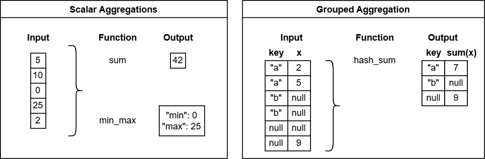
Figure 6.1 – Depiction of aggregation functions

There are also grouped aggregation functions, which are the equivalent of a SQL-style group by operation. Instead of an operation on all the values in the input, grouped aggregations first partition by a specified key column, and then output a single scalar value per group in the input.

Some examples are hash_max, hash_product, and hash_any.

Element-wise or scalar functions

Unary or single-input functions in this category operate on each element of the input separately. A scalar input produces a scalar output and array inputs produce array outputs.

Some examples are abs, negate, and round. See Figure 6.2:

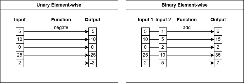
Figure 6.2 – Depiction of scalar functions

Binary functions in this category operate on aligned elements between the inputs, such as adding two arrays. Two scalar inputs produce a scalar output, while two array inputs must have the same length and produce an array output. Providing one scalar and one array input will perform the operation as if the scalar were an array of the same length, N, as the other input, with the value repeated.

Some examples are add, multiply, shift_left, and equal.

Array-wise or vector functions

Functions in this category use the entire array for their operations, frequently performing transformations or outputting a different length than the input array. See Figure 6.3.

Some examples are unique, filter, and sort_indices:

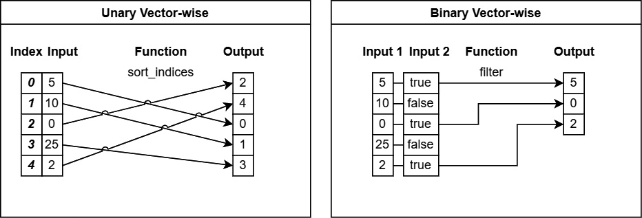
Figure 6.3 – Depiction of vector functions

Now that we've explained the concepts, let's learn how to execute the computation functions on some data!

Executing compute functions

The Arrow compute library has a global FunctionRegistry, which allows looking up functions by name and listing what is available to call. The list of available compute functions can also be found in the Arrow documentation at https://arrow.apache.org/docs/cpp/compute.html#available-functions. Let's see how to execute these functions now!

Using the C++ compute library

The compute library is managed as a separate module in the base Arrow package. If you've compiled the library yourself from source, make sure that you've used the ARROW_COMPUTE=ON option during configuration.

Example 1 – adding a scalar value to an array

Our first example is going to be a simple scalar function call on an array of data, using the same Parquet file as we did previously in the C Data API examples:

1. First things first, we need to read the column we want from the Parquet file. We can use the Parquet C++ library to open the file and it provides an adapter for direct conversion to Arrow objects from Parquet:

   #include <arrow/io/file.h>

   #include <arrow/status.h>

   #include <parquet/arrow/reader.h>

   ...

   constexpr auto filepath = "<path to file>/yellow_tripdata_2015-01.parquet";

   auto input = arrow::io::ReadableFile::Open(filepath).ValueOrDie();

   std::unique_ptr<parquet::arrow::FileReader> reader;

   arrow::Status st = parquet::arrow::OpenFile(input,

                         arrow::default_memory_pool(),

                         &reader);

   if (!st.ok()) {

       // handle the error

   }

2. After opening the file, the easy solution would be to just read the whole file into memory as an Arrow table, which is what we will do here. Alternately, you could read only one column from the file if you prefer using the ReadColumn function:

   std::shared_ptr<arrow::Table> table;

   st = reader->ReadTable(&table);

   if (!st.ok()) {

       // handle the error

   }

   std::shared_ptr<arrow::ChunkedArray> column =

                 table->GetColumnByName("total_amount");

   std::cout << column->ToString() << std::endl;

3. Now that we have our column, let's add the value 5.5 to each element in the array. Because addition is a commutative operation, the order of the arguments doesn't matter when passing the scalar and column objects. If we were instead performing subtraction, for example, the order would matter and be reflected in the result:

   #include <arrow/compute/api.h>

   #include <arrow/scalar.h>

   #include <arrow/datum.h>

   ...

   arrow::Datum incremented = arrow::compute::CallFunction("add",

         {column, arrow::MakeScalar(5.5)}).ValueOrDie();

   std::shared_ptr<arrow::ChunkedArray> output =

         std::move(incremented).chunked_array();

   std::cout << output->ToString() << std::endl;

4. Finally, we just need to compile this. As before, we'll use pkg-config to generate our compiler and linker flags on the command line to make life easier:

   $ g++ compute_functions.cc -o example1 'pkg-config --cflags --libs parquet arrow-compute'

5. When we run our mainprog, we can see the output to confirm that it worked. In the preceding code snippets, we printed out the column of data both before and after we added the scalar value 5.5 to it, allowing us to directly see that it worked:

   $ ./example1

   [

   [

     17.05,

     17.8,

     10.8,

     4.8,

     <values removed for brevity>

   ]

   ]

   [

   [

     22.55,

     23.3,

     16.3,

     10.3,

     <values removed for brevity>

   ]

   ]

   Note

   Notice in the code snippets that we are using arrow::ChunkedArray instead of arrow::Array. Remember what a chunked array is from Chapter 2, Working with Key Arrow Specifications? Because Parquet files can be split into multiple row groups, we can avoid copying data by using a chunked array to treat the collection of one or more discrete arrays as a single contiguous array. Arrow table objects allow each individual column to also be chunked, potentially with different chunk sizes between them. Not all compute functions can operate on both chunked and non-chunked arrays, but most can. If your input is a chunked array, your output will be chunked also.

While we used arrow::compute::CallFunction in the preceding example, many functions also have convenient concrete APIs that are available to call. In this case, we could have used arrow::compute::Add(column, arrow::MakeScalar(5.5)) instead.

Example 2 – min-max aggregation function

For our second example, we're going to compute the minimum and maximum values of the total_amount column from the file. Instead of outputting a single scalar number, this will produce a scalar structure that contains two fields. Always look at the documentation to see what the return value looks like for the compute functions:

1. Open the Parquet file and retrieve the total_amount column as before. Consult the previous example's steps 1 and 2 if you need to. I trust you.
2. Some functions, such as the min_max function, accept or require an options object, which can affect the behavior of the function. The return value is a scalar struct containing fields named min and max. We just need to cast the Datum object to StructScalar to access it:

   arrow::compute::ScalarAggregateOptions scalar_agg_opts;

   scalar_agg_opts.skip_nulls = false;

   arrow::Datum minmax = arrow::compute::CallFunction("min_max",

           {column}, &scalar_agg_opts).ValueOrDie();

   std::cout <<

       minmax.scalar_as<arrow::StructScalar>().ToString()

             << std::endl;

3. Compile with the same options as before and you should get the following output when running it:

   $ g++ examples.cc -o example2 'pkg-config --cflags --libs parquet arrow-compute'

   $ ./example2

   {min:double = -450.3, max:double = 3950611.6}

Did you get the same output I did? Getting the hang of calling different functions by name and using the documentation to determine the data types yet? Let's keep going!

Example 3 – sorting a table of data

Our last example is of a vector compute function, sorting the entire table of data by the total_amount column:

1. Once again, open the file and read it into arrow::Table like we did in the previous two examples.
2. Create the sort options object to define what column we want to sort the table by and the direction to sort:

   arrow::compute::SortOptions sort_opts;

   sort_opts.sort_keys = { // one or more key objects

       arrow::compute::SortKey{"total_amount",

          arrow::compute::SortOrder::Descending}};

   arrow::Datum indices = arrow::compute::CallFunction(

              "sort_indices", {table},

               &sort_opts).ValueOrDie();

3. The sort_indices function on its own doesn't do any copying of data; however, the output is an array of the row indices of the table, which define the sorted order. We could take the array of indices and build our new sorted version of the table if we wanted, but we can instead let the Compute API do that for us!

   arrow::Datum sorted = arrow::compute::Take(table, indices).ValueOrDie();

   // or you can use CallFunction("take", {table, indices})

   auto output = std::move(sorted).table();

The take function takes an array, chunked array, record batch, or table for the first argument and an array of numeric indices as the second argument. For each element in the array of indices, the value at that index in the first argument is added to the output. In our example, it's using the generated list of sorted indices to output the data in sorted order. Since we gave it a table as input, it outputs a table. The same would happen for a record batch, array, or chunked array.

Try playing around with different functions and compute functionality to see what the outputs look like and what options are available for customizing the behavior, such as whether null values should be placed at the beginning or end when sorting. As an exercise, try sorting a table of data by multiple keys in different directions or performing different transformations of the data, such as filtering or producing derived computations. Then, we can move on to performing the same examples but using Python.

Using the compute library in Python

The compute library is also made available to Python as part of the pyarrow module. Python's syntax and ease of use make it even simpler to utilize than the C++ library. Many of the functions that you may convert to pandas DataFrames or use NumPy for are made accessible directly on the Arrow data using the compute library, saving you precious CPU cycles from having to convert between formats.

Example 1 – adding a scalar value to an array

Just like the C++ examples, we'll start with adding a scalar value to the total_amount column from the NYC trip data Parquet file:

1. Do you remember how to read a column from a Parquet file using Python? I'll recap it here just in case you don't:

   >>> import pyarrow.parquet as pq

   >>> filepath = '<path to file>/yellow_tripdata_2015-01.parquet'

   >>> tbl = pq.read_table(filepath) # read the entire file in

   >>> tbl = pq.read_table(filepath, columns=['total_amount']) # read just the one column

   >>> column = tbl['total_amount']

2. The pyarrow library will perform a lot of the necessary type casting for you, making it very easy to use the Compute API with it:

   >>> import pyarrow.compute as pc

   >>> pc.add(column, 5.5)

   <pyarrow.lib.ChunkedArray object at 0x7fdd2a3719a0>

   [

     [

       22.55,

       23.3,

       16.3,

       10.3,

   ...

The arguments can be native Python values, pyarrow.Scalar objects, arrays, or chunked arrays. The library will cast accordingly as best it can if necessary.

Example 2 – min-max aggregation function

Continuing the tour, we can find the minimum and maximum values just like we did in C++:

Get our column of data from the Parquet file just like in the previous example. Try to figure it out yourself before looking at the following code snippet. I promise you that it's very easy:

>>> pc.min_max(column)

<pyarrow.StructScalar: [('min', -450.3), ('max', 3950611.6)]>

As expected, the values match those that were computed in the C++ version.

Example 3 – sorting a table of data

To complete our examples, we will sort the entire table of data in the Parquet file. Try figuring it out yourself before following the steps, then see whether you're right:

1. Once again, read the whole Parquet file in using the read_table function.
2. Are you ready for this? While the compute library has a take function, there's one directly exposed on the Table object itself in the Python library, making this easier:

   >>> sort_keys = [('total_amount', 'descending')]

   >>> out = tbl.take(pc.sort_indices(tbl, sort_keys=sort_keys)

That's it! The sort keys are defined similarly to the C++ as a tuple of the column name and the direction to sort in. Other options can be passed by instead using the full pc.SortOptions object and passing that to sort_indices using the options keyword instead of sort_keys.

Given the ease of use and convenience of the compute library, you might wonder how it stacks up against just performing simple computations yourself. For instance, does it make more sense to manually write a loop to add a constant to an Arrow array or should you always use the compute library? Well, let's take a look…

Picking the right tools

The Arrow compute libraries provide an extremely easy-to-use interface, but what about performance? Do they exist just for ease of use? Let's try it out and compare!

Adding a constant value to an array

For our first test, let's try adding a constant value to a sample array we construct. It doesn't need to be anything extravagant, so we can create a simple 32-bit integer Arrow array and then add 2 to each element and create a new array. We're going to create arrays of various sizes and then see how long it takes to add a constant value of 2 to the Arrow array using different methods.

Remember!

Semantically, an Arrow array is supposed to be immutable, so adding a constant produces a new array. This property of immutability is often used to create optimizations and reusability of memory depending on the particular Arrow implementation. While it is possible to potentially achieve greater performance by modifying a buffer in place, care must be taken if you choose to do that. Ensure that there are no other Arrow array objects that also share the same buffers of memory; otherwise, you can end up shooting yourself in the foot.

First thing's first: we need to create our test array. Let's do that!

#include <numeric> // for std::iota

std::vector<int32_t> testvalues(N);

std::iota(std::begin(testvalues), std::end(testvalues), 0);

arrow::Int32Builder nb;

nb.AppendValues(testvalues);

std::shared_ptr<arrow::Array> numarr;

nb.Finish(&numarr);

auto arr = std::static_pointer_cast<arrow::Int32Array>(numarr);

Pretty simple, right? In the first highlighted line, we utilize std::iota to fill the vector with the range of values between 0 and N. Then, we append these values to an Int32Builder object in the second highlighted line to create our test array.

There are four cases we're going to test:

• Using the arrow::compute::Add function
• A simple for loop with arrow::Int32Builder
• Using std::for_each with arrow::Int32Builder, calling Reserve on the builder to pre-allocate the memory
• Treating the raw buffer as a C-style array, pre-allocating a new buffer, and constructing the resulting Arrow array from the buffers

We're going to walk through the code for each of these first, then we'll run each of them with different length arrays by changing the value of N. We'll use our trusty timer class from previous examples, like in Chapter 3, Data Science with Apache Arrow, to time how long it takes. (You can find the timer.h file in this book's GitHub repository: https://github.com/PacktPublishing/In-Memory-Analytics-with-Apache-Arrow-/blob/main/chapter6/cpp/timer.h.) Let's see what patterns we can observe!

Compute Add function

This is our simplest case, showcasing the ease of use of the compute library. Give it a try yourself before looking at the code snippet:

arrow::Datum res1;

{

    timer t;

    res1 = cp::Add(arr, arrow::Datum{(int32_t)2}).    MoveValueUnsafe();

}

What do you think? Short and sweet! We declare arrow::Datum outside of the scope so that we can hold onto it and verify that our other approaches produce the same result.

A simple for loop

For this case, we'll just create an Int32Builder object and iterate the array, calling Append and AppendNull. This is the naive solution that someone would likely come up with if asked to perform the addition of a constant to an Arrow array:

arrow::Datum res2;

{

    timer t;

    arrow::Int32Builder b;

    for (size_t i = 0; i < arr->length(); ++i) {

        if (arr->IsValid(i)) {

            b.Append(arr->Value(i)+2);

        } else {

            b.AppendNull();

        }

    }

    std::shared_ptr<arrow::Array> output;

    b.Finish(&output);

    res2 = arrow::Datum{std::move(output)};

}

std::cout << std::boolalpha << (res1 == res2) << std::endl;

Not too bad, right? That final highlighted line will output true if the result generated is equal to our previous result and false if it is not. Onward!

Using std::for_each and reserve space

This implementation is mostly a variation on the previous for loop solution, with some pre-allocation of memory. We're just going to utilize std::for_each and a lambda function instead. For this solution, we're going to need a couple of extra headers:

#include <arrow/util/optional.h> 

#include <algorithm>

Now, the implementation:

arrow::Datum res3;

{

    timer t;

    arrow::Int32Builder b;

    b.Reserve(arr->length());

    std::for_each(std::begin(*arr), std::end(*arr),

         [&b](const arrow::util::optional<int32_t>& v) {

             if (v) { b.Append(*v + 2); }

             else { b.AppendNull(); }

         });

    std::shared_ptr<arrow::Array> output;

    b.Finish(&output);

    res3 = arrow::Datum{std::move(output)};               

}

std::cout << std::boolalpha << (res1 == res3) << std::endl;

Notice that the highlighted lines are pretty much the only changes (outside of assigning to res3 instead of res2). Here, we're taking advantage of the fact that Arrow arrays provide stl-compatible iterators, using arrow::util::optional<T> as value_type they return. This is convenient because the optional class can be coerced to be a Boolean to check whether it is null, and overloads the * operator to retrieve the actual value. Now the last one…

Divide and conquer

For this implementation, we take advantage of a few elements of the Arrow specification. Consider these premises:

• For indexes that are null, the value in the raw data buffer can be literally anything.
• A primitive numeric array contains two buffers, a bitmap and a buffer containing the raw data.
• When adding a constant to an Arrow array, the resulting array's null bitmap would be identical to the original array.

Given these three premises, we can divide and process the array's null bitmap and data buffer separately. Since this example is a bit more complex, we'll break it up more to make it easier to explain:

1. We start the same as the previous examples, creating  Datum and a timer inside of a nested scope:

   arrow::Datum res4;

   {

       timer t;

2. Next, we allocate a buffer to hold the resulting data. Since we know the length of the array, we can multiply it by the size of a 32-bit integer to determine the total number of bytes to allocate. Then, we use reinterpret_cast to acquire a pointer to the allocated memory, which we can treat as a C-style array:

       std::shared_ptr<arrow::Buffer> new_buffer =

          arrow::AllocateBuffer(sizeof(int32_t)*arr->length())

            .MoveValueUnsafe();

       auto output = reinterpret_cast<int32_t*>(

          new_buffer->mutable_data());

3. Now, we just use std::transform to add a constant of 2 to every element in the array, regardless of whether or not it is null:

       std::transform(arr->raw_values(),

                      arr->raw_values() + arr->length(),

                      output,

                      [](const int32_t v) {

                         return v + 2;

                      });

4. Finally, we reference the existing null bitmap and create our new array using the new buffer:

        res4 = arrow::Datum{arrow::MakeArray(

          arrow::ArrayData::Make(

             arr->type(), arr->length(),

             std::vector<std::shared_ptr<arrow::Buffer>>{

                    arr->null_bitmap(), new_buffer},

            arr->null_count()))};

   }

   std::cout << std::boolalpha << (res1 == res4) << std::endl;

Did you follow all that? If not, have a look at Figure 6.4:

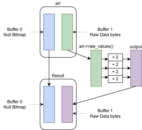
Figure 6.4 – Divide and conquer compute

You can see in Figure 6.4 where each of the variables fits in the diagram, hopefully painting a clear picture of how we split up and processed the two buffers separately to create the new array.

Now, the moment of truth. Let's compare the performance of these approaches! Figure 6.5 is a graph showing the performance of each one:

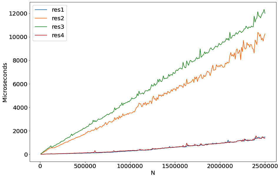
Figure 6.5 – Performance of adding a constant to an int32 array

To create this chart, I smoothed any outliers by running each approach in a loop numerous times and then dividing the time it took by the number of iterations. This is a standard benchmarking approach. It's pretty clear that not only does the compute library provide an easy-to-use interface, but it's also extremely performant. Of the different methods we tried, the only one that was on par with just calling the Add function of the compute library was our divide and conquer approach. This makes sense because it's actually the same underlying strategy that the compute library uses! This is awesome when dealing with a single table of data, but most modern datasets aren't quite so simple. When you're dealing with multifile datasets of tabular data, you'll need some extra utilities.

Summary

The compute APIs aren't just a convenient interface for performing functions on Arrow-formatted data but are also highly performant. The goal of the library is to expose highly optimized computational functions for as many use cases as possible in an easy-to-use way. The functions that it exposes are also highly composable as we saw with the examples for sorting a table.

Between this chapter and the previous one, Chapter 5, Crossing the Language Barrier with the Arrow C Data API, we've explored the building blocks of any analytical engine. Both the Arrow C data interface and the compute APIs are extremely useful in different use cases and even in conjunction with one another. For example, let's say you're using Arrow in a language that doesn't yet expose the compute APIs. By using the C Data API, you can efficiently share the data with another component that has access to the compute APIs.

Now, if you're dealing with multifile datasets of tabular data, which might be larger than the available memory on a single machine, you can still use the compute libraries. This is what we're going to cover next in Chapter 7, Using the Arrow Datasets API. The datasets library can do a lot of the heavy lifting for you in reading, selecting, filtering, and performing computations on data in a streaming fashion.

Onward and upward! To the cloud!