Chapter 2: Working with Key Arrow Specifications

Utilities to perform analytics and computations are only useful if you have data to perform them on. That data can live in many different places and formats, both local and remote to the machine being used to analyze it. The Arrow libraries provide a bunch of functionalities that we'll cover for reading data from and interacting with multiple different formats in multiple different locations. Now that you have a solid understanding of what Arrow is and how to manipulate arrays, in this chapter, you will learn how to get data into the Arrow format and communicate it between different processes.

In this chapter, we're going to cover the following topics:

• Importing data from multiple formats, including CSV, Apache Parquet, and pandas DataFrames
• Interactions between Arrow and pandas data
• Utilizing shared memory for near zero-cost data sharing

Technical requirements

Throughout this chapter, I'll be providing various code samples while using the Python, C++, and Golang Arrow libraries and the public NYC Taxi Trip Duration dataset.

To run the practical examples in this chapter, you will need the following:

• A computer that's connected to the internet
• Your preferred IDE (VS Code, Sublime, Emacs, Vim, and so on)
• Python 3+ with the pyarrow and pandas modules installed
• Go 1.16+
• A C++ compiler (capable of compiling C++11 or newer) with the Arrow libraries installed
• The sample_data folder from this book's GitHub repository: https://github.com/PacktPublishing/In-Memory-Analytics-with-Apache-Arrow-

Let's get started!

Playing with data, wherever it might be!

Modern data science, machine learning, and other data manipulation techniques frequently require data to be merged from multiple locations to perform tasks. Often, this data isn't locally accessible but rather is stored in some form of cloud storage. Most of the implementations of the Arrow libraries provide native support for local filesystem access, AWS Simple Storage Service (S3), and Hadoop Distributed File System (HDFS). In addition to the natively supported systems, filesystem interfaces are generally implemented or used in language-specific cases to make it easy to add support for other filesystems.

Once you're able to access the platform your files are located on (whether that is local, in the cloud, or otherwise), you need to make sure that the data is in a format that is supported by the Arrow libraries for importing. Check the documentation for the Arrow library of your preferred language to see what data formats are supported. The abstractions provided by the Arrow libraries make it very easy to create a single process for manipulating data that will work regardless of the location or format of that data, and then write it out to different formats wherever you'd like. The following diagram only shows a few data formats that are supported by most Arrow libraries, but remember, just because a format isn't listed doesn't necessarily mean it's not supported:

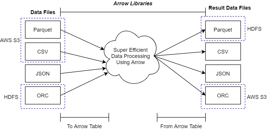
Figure 2.1 – Using Arrow libraries with data files

In the preceding diagram, the dotted outlines point out how the data files may exist in one location before they are processed (such as in S3 or an HDFS cluster); the result of this processing can be written out to an entirely different storage location and format.

To provide optimized and consistent usage of the library functions, and for ease of implementation, many Arrow libraries define specific interfaces for filesystem usage. The exact nature of these interfaces will differ from language to language, but all of them are used to abstract away the particulars of the filesystem when it's interacting with imported data files. Before we jump into working with data files directly, we need to introduce a couple of important Arrow concepts. We covered Arrow arrays and record batches in Chapter 1, Getting Started with Apache Arrow, so let's introduce chunked arrays and tables.

Working with Arrow tables

To quickly review, a record batch is a collection of equal length Arrow arrays along with a schema describing the columns in terms of names, types, and metadata. Often, when reading in and manipulating data, we get that data in chunks and then want to assemble it to treat it as a single large table, as shown in the following diagram:

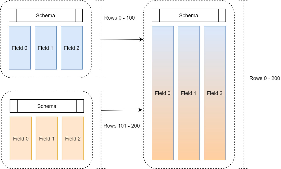
Figure 2.2 – Multiple record batches

One way to do this would be to simply allocate enough space to hold the full table and then copy the columns of each record batch into the allocated space. That way, we end up with the finished table as a single cohesive record batch in memory. There are two big problems with this method that prevent it from being scalable:

• It's potentially very expensive to both allocate an entirely new large chunk of memory for each column and copy all the data over.
• What if we get another record batch of data? We would have to do this again to accommodate the – now larger – table each time we get more data.

This is where the concept of chunked arrays comes to the rescue, as shown in the following diagram:

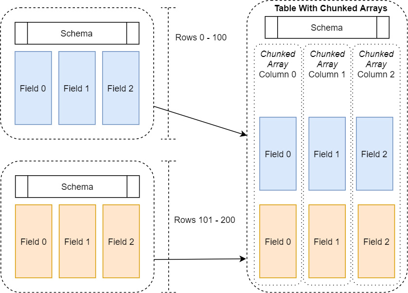
Figure 2.3 – Table with chunked arrays

A chunked array is just a thin wrapper around a group of Arrow arrays of the same data type. This way, we can incrementally build up an array, or even a whole table, efficiently without constantly having to allocate larger and larger chunks of memory and copying data. In the same manner, an Arrow table holds one or more chunked arrays and a schema, very similar to how a record batch holds regular Arrow arrays and a schema. The table allows us to conceptually treat all the data as if it were a single contiguous table of data, without having to pay the costs to frequently reallocate and copy the data.

Of course, there are trade-offs to this: we lose some of our memory locality by no longer having the arrays as fully contiguous buffers. You want these chunks to be as large as possible to get as much benefit from the locality when processing the data as possible, which means it's a balancing act. You need to balance the cost of the allocations and copies against the cost of processing non-contiguous data. Thankfully, most of this complexity is handled by the Arrow libraries themselves under the hood in the I/O interfaces when reading in data to process. But understanding these concepts is key to getting the best performance possible for your dataset and operations.

With that out of the way, let's start reading and writing some files!

In the interests of brevity, we're just going to focus on Python and C++ in this section. But fear not! Golang will pop up in other examples as we go. In the next section, we're going to look at how to utilize the available filesystem interfaces to import data from the different supported file formats. First up is Python!

Accessing data files with pyarrow

The Python Arrow library defines a base class interface and then provides a few concrete implementations of that interface for different locations to access files, as shown in the following diagram:

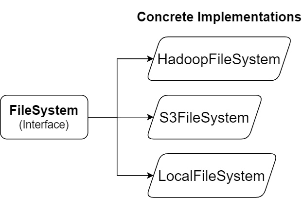
Figure 2.4 – Python Arrow filesystem interfaces

The abstract interface, FileSystem, provides utilities both for input and output streams and for directory operations. Abstracting out the underlying implementation of the filesystem interactions provides a single interface that simplifies the view of the underlying data storage. Regardless of the system, the paths will always be separated by forward slashes (/), leave out the special path components such as . and .., and only expose basic metadata about the files, such as their size and last modification time. When constructing a FileSystem object, you can either construct the type you need explicitly or allow inference from the URI, like so:

• Local Filesystem: The constructor for LocalFileSystem takes a single optional argument, use_mmap. It defaults to being false, but if set to true, it will memory map files when opening them. The implications of memory mapping the file will be covered in Chapter 4, Format and Memory Handling, in the Learning memory cartography section. Let's construct the object:

  >>> from pyarrow import fs

  >>> local = fs.LocalFileSystem() # create local file system instance

  >>> f, p = fs.FileSystem.from_uri('file:///home/mtopol/')

  >>> f

  <pyarrow._fs.LocalFileSystem object at 0x0000021FAF8F6570>

  >>> p

  '/home/mtopol/'

Standard Windows paths, such as C:Usersmtopol..., will not work due to the colon present in them. Instead, you can specify such a path as a URI with forward slashes: file:///c/Users/mtopol/….

• AWS S3: The constructor for S3FileSystem allows you to specify your credentials, if necessary, through multiple arguments in addition to other connection properties such as the region or endpoint overrides. Alternatively, the constructor will also inspect the standard S3 credential configurations, such as environment variables like AWS_ACCESS_KEY_ID or the ~/.aws/config file:

  >>> from pyarrow import fs

  >>> s3 = fs.S3FileSystem(region='us-east-1') # explicit create

  >>> s3, path = fs.FileSystem.from_uri('s3://my-bucket/')

  >>> s3

  <pyarrow._s3fs.S3FileSystem object at 0x0000021FAF7F99F0>

  >>> path

  'my-bucket'

• HDFS: Using HDFS gets a little tricky as it requires having the Java Native Interface (JNI) libraries on your path so that they can be loaded. JNI is a framework that allows Java code running in the Java Virtual Machine (JVM) to call, and get called by, applications and libraries native to the platform it is running on. I won't cover installing HDFS here, but the important pieces necessary for being able to use it with pyarrow are libjvm.so and libhdfs.so. Both of these must be in $LD_LIBRARY_PATH (just $PATH on Windows and $DYLD_FALLBACK_LIBRARY_PATH on newer macOS releases) so that they can be loaded at runtime. Provided these libraries are accessible at runtime, you can communicate with an HDFS cluster with pyarrow:

  >>> from pyarrow import fs

  >>> hdfs = fs.HadoopFileSystem(host='namenode', port=8020)

  >>> hdfs, path = fs.FileSystem.from_uri('hdfs://namenode:8020/tmp')

  >>> hdfs

  <pyarrow._hdfs.HadoopFileSystem object at 0x7f7a70960bf0>

  >>> path

  '/tmp'

pyarrow will attempt to connect to the HDFS namenode upon construction and will fail if it's not successful. The runtime lookup of the Hadoop libraries depends on a couple different environment variables. If the library isn't in your LD_LIBRARY_PATH, you can use the following environment variables to configure how it is looked up.

If you have a full Hadoop installation, you should have HADOOP_HOME defined, which usually has lib/native/libhdfs.so. JAVA_HOME should be defined to point to your Java SDK installation. If libhdfs.so is installed somewhere other than $HADOOP_HOME/lib/native, you can specify the explicit location with the ARROW_LIBHDFS_DIR environment variable.

Many of the I/O-related functions in pyarrow allow a caller to either specify a URI, inferring the filesystem, or have an explicit argument that allows you to specify the FileSystem instance that will be used. Once you have initialized your desired filesystem instance, the interface can be utilized for many standard filesystem operations, regardless of the underlying implementation. Here's a subset of the abstracted functions to get you started:

• create_dir: Create directories or subdirectories
• delete_dir: Delete a directory and its contents recursively
• delete_dir_contents: Delete a directory's contents recursively
• copy_file, delete_file: Copy or delete a specific file by path
• open_input_file: Open a file for random access reading
• open_input_stream: Open a file for only sequential reading
• open_append_stream: Open an output stream for appending data
• open_output_stream: Open an output stream for sequential writing

In addition to manipulating files and directories, you can also use the abstraction to inspect and list the contents of files and directories. Opening files or streams produces what's referred to as a file-like object, which can be used with any functions that work with such objects, regardless of the underlying storage or location.

At this point, you should have a firm grasp of how to open and refer to data files using the Python Arrow library. Now, we can start looking at the different data formats that are natively implemented and how to process them into memory as Arrow arrays and tables.

Working with CSV files in pyarrow

One of the most ubiquitous file formats to be used with data is a delimited text file such as a comma-separated values or CSV file. In addition to commas, they are also often used as tab or pipe delimited files. Because the raw text of a CSV file doesn't have well-defined types, the Arrow library makes attempts to guess the types and provides a multitude of options for parsing and converting the data into or out of Arrow data when reading or writing. More information about how type inference is performed can be found in the Arrow documentation: https://arrow.apache.org/docs/python/csv.html#incremental-reading.

The default options for reading in CSV files are generally pretty good at inferring the data types, so reading simple files is easy. We can see this by using the train.csv sample data file, which is a subset of the commonly used NYC Taxi Trip dataset:

>>> import pyarrow as pa

>>> import pyarrow.csv

>>> table = pa.csv.read_csv('sample_data/train.csv')

>>> table.schema

vendor_id: string

pickup_at: timestamp[ns]

dropoff_at: timestamp[ns]

passenger_count: int64

trip_distance: double

pickup_longitude: double

pickup_latitude: double

rate_code_id: int64

store_and_fwd_flag: string

dropoff_longitude: double

dropoff_latitude: double

payment_type: string

fare_amount: double

extra: double

mta_tax: double

tip_amount: double

tolls_amount: double

total_amount: double

The first thing to note is that we pass a string directly into the read_csv function. Like many of the Python Arrow file reading functions, it can take either of the following as its argument:

• string: A filename or a path to a file. The filesystem will be inferred if necessary.
• file-like object: This could be the object that's returned from the built-in open function or any of the functions on a FileSystem that returns a readable object, such as open_input_stream.

The first line of the file contains the column headers, which are automatically used as the names of the columns for the generated Arrow table. After that, we can see that the library recognizes the timestamp columns from the values, even determining the precision to be in seconds as opposed to milliseconds or nanoseconds. Finally, you can see the numeric columns versus string columns, which determines the columns being doubles instead of integer columns.

Reading in a CSV file returns an object of the pyarrow.Table type that contains a list of pyarrow.lib.ChunkedArray objects. This follows the pattern mentioned earlier regarding tables and chunked arrays. When you're reading in the file, it can be parallelized by reading groups of rows at a time and then building the chunked columns without having to copy data around. The following diagram shows a parallelized file read:

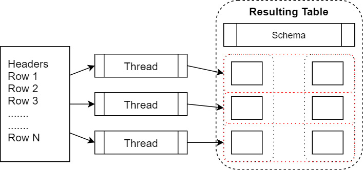
Figure 2.5 – Parallelized file read

Here, we can see threads parallelizing the reads from a file. Each thread reads in a group of rows into array chunks. These are then added to the columns of the table as a zero-copy operation once the Arrow arrays have been created. We can examine the columns of the finished table in the Python interpreter to see this in action:

>>> table.column(0).num_chunks

192

>>> table.column(0).chunks

[<pyarrow.lib.StringArray object at 0x000001B2C5EB9FA8>

[

  "VTS",

  "VTS",

  "VTS",

  "VTS",

  "VTS",

  "VTS",

  "VTS",

  ...

  "CMT",

  "VTS",

  "VTS",

  "VTS",

  "VTS",

  "VTS",

  "CMT",

  "VTS",

  "VTS",

  "VTS"

], <pyarrow.lib.StringArray object at 0x000001B2C5EBB048>

[……

In addition to the input stream or filename, the CSV reading functions have three types of options that can be passed in – ReadOptions, ParseOptions, and ConvertOptions. Each of these has a set of options to control the different aspects of reading the file and creating the Arrow table object, as follows:

• ReadOptions: This allows you to configure whether you should use threads for reading, the block size to read in at a time, and how to generate the column names for the table either by reading from the file, providing them directly, or auto-generating them:

  # if the extension is a recognized compressed format extension

  # the data will automatically be decompressed during reading

  table = pa.csv.read_csv('file.csv.gz', read_options=pa.csv.ReadOptions(

       encoding='utf8', # encoding type of the file

       column_names=['col1', 'col2', 'col3'],

       block_size=4096, # number of bytes to process at a time

  )

• ParseOptions: This controls the delimiter to use when you're figuring out the columns, quote and escape characters, and how to handle newlines:

  table = pa.csv.read_csv(input_file, parse_options=pa.csv.ParseOptions(

        delimiter='|', # for a pipe delimited file

        escape_char='', # allow backslash to escape values

      )

• ConvertOptions: This provides various options for how to convert the data into Arrow array data, including specifying what strings should be considered null values, which strings should be considered true or false for Boolean values, and various other options for how to parse strings into Arrow data types:

  table = pa.csv.read_csv('tips.csv', convert_options=pa.csv.ConvertOptions(

         column_types={

             'total_bill': pa.decimal128(precision=10, scale=2),

             'tip': pa.decimal128(precision=10, scale=2),

         },

         # only read these columns from the file, in this order

         # leaving out any other columns

         include_columns=['tip', 'total_bill', 'timestamp'],

  )

In addition to all the functionality for reading CSV files, there is a write_csv function for writing a CSV file from a record batch or table. Just as with the read function, it takes a filename or path or a file-like object that it can write to as an argument. There are only two available options for manipulating the write – include the initial header line with the names of the columns or include the batch size to use when writing out rows. Here's a simple example of a function that can read in a CSV file and write a subset of columns out to a new file:

def create_subset_csv(input, output, column_names):

    table = pa.csv.read_csv(input,

                            convert_options=pa.csv.ConvertOptions(

                                include_columns=column_names))

    pa.csv.write_csv(table, output,

                     write_options=pa.csv.WriteOptions(

                                     include_header=True))

In some situations, you may want to write data out to a CSV file incrementally as you generate or retrieve the data. When you're doing this, you don't want to keep the entire table in memory at once if you can avoid it. Here, you can use pyarrow.csv.CSVWriter to write data incrementally:

schema = pa.schema([("col", pa.int64())])

with pa.csv.CSVWriter("output.csv", schema=schema) as writer:

    for chunk in range(10):

        datachunk = range(chunk*10, (chunk+1)*10)

        table = pa.Table.from_arrays([pa.array(datachunk)],

                                     schema=schema)

        writer.write(table)

The next data format we're going to cover is another very common one: JSON data.

Working with JSON files in pyarrow

The expected format for JSON data files is that they are line delimited files where each line is a JSON object containing a single row of data. The process of reading JSON files is nearly identical to reading in CSV files! The following is a sample JSON data file:

{"a": 1, "b": 2.0, "c": 1}

{"a": 3, "b": 3.0, "c": 2}

{"a": 5, "b": 4.0, "c": 3}

{"a": 7, "b": 5.0, "c": 4}

Reading this file into a table is simple:

>>> import pyarrow as pa

>>> import pyarrow.json

>>> table = pa.json.read_json(filename)

>>> table.to_pydict()

{'a': [1, 3, 5, 7], 'b': [2.0, 3.0, 4.0, 5.0], 'c': [1, 2, 3, 4]}

Just like reading in a CSV file, there are ReadOptions and ParseOptions available that allow you to configure the behavior for creating the Arrow data. You can do this by specifying an explicit schema and defining how to handle unexpected fields. Currently, there is no corresponding write_json function.

Working with ORC files in pyarrow

Unlike the JSON and CSV formats, the Apache Optimized Row Columnar (ORC) format isn't as popular unless you already work with the Hadoop data ecosystem. Apache ORC is a row-column format that was originally developed by Hortonworks for storing data in a compressed format so that it can be processed by Apache Hive and other Hadoop utilities. It stores data in a column-oriented format in conjunction with file indexes and splits the file into stripes to facilitate predicate pushdown and optimized reads.

Since the ORC file format is used frequently for data storage and querying, the pyarrow library provides an interface for reading ORC files directly into an Arrow table, aptly named pyarrow.orc.ORCFile. Like Arrow, ORC files have a schema, and the columns are specifically typed, allowing them to be easily converted. This is because no ambiguity exists like when you're trying to infer data types from a JSON or CSV file.

Note

The orc module in pyarrow is not currently included in the Windows build of the Python package wheels. If you're on Windows, you'll have to build it yourself from the source.

Let's adjust our previous examples so that it reads an ORC file rather than a CSV or JSON file:

1. To read an ORC file into one or more Arrow tables, first, create an ORCFile instance:

   >>> import pyarrow as pa

   >>> import pyarrow.orc

   >>> of = pa.orc.ORCFile('train.orc')

   >>> of.nrows

   1458644

   >>> of.schema

   vendor_id: string

   pickup_at: timestamp[ns]

   dropoff_at: timestamp[ns]

   passenger_count: int64

   trip_distance: double

   pickup_longitude: double

   pickup_latitude: double

   rate_code_id: int64

   store_and_fwd_flag: string

   dropoff_longitude: double

   dropoff_latitude: double

   payment_type: string

   fare_amount: double

   extra: double

   mta_tax: double

   tip_amount: double

   tolls_amount: double

   total_amount: double

As with CSV and JSON files, the argument for creating an ORCFile can be a file path or a file-like object.

2. With the object, you can now read either a single stripe or the entire file into an Arrow table, including reading only a subset of the columns if desired:

   >>> tbl = of.read(columns=['vendor_id', 'passenger_count', 'rate_code_id']) # leave this out or use None to get all cols

   >>> tbl

   pyarrow.Table

   vendor_id: string

   passenger_count: int64

   rate_code_id: int64

   ---

   id: [["VTS","VTS","VTS","VTS","VTS",…]]

   passenger_count: [[1,1,2,1,1,1,1,1,1,2,...,5,5,1,1,1,3,5,4,1,1]]

   trip_duration: [[1,1,1,1,1,…,1,1,1,1,1,1,1]]

Along with reading an ORC file, we can also write to an ORC file using pyarrow.orc.write_table. The arguments for this write_table method are the table to write and the location of the file to write. The last file format that we're going to cover with the pyarrow library is Apache Parquet.

Working with Apache Parquet files in pyarrow

If you're not familiar with it, Parquet is similar to ORC as both are column-oriented, on-disk storage formats with compression. Both also contain various kinds of metadata to make querying directly from the files more efficient. Think of them as two different flavors of column-based storage with different trade-offs made in their designs.

Note

With all these columnar-based storage formats, you may be wondering why Arrow exists and when to use which format and for what reasons. Well, don't worry! We'll dig into answering these questions, along with other format comparison questions, later in Chapter 4, Format and Memory Handling.

At this point, you've probably picked up the pattern in the library design here and can guess what it may look like to read a Parquet file into an Arrow table. Go ahead – sketch out what you think the Python code may look like; I'll wait.

Got something? Okay then, let's take a look:

>>> import pyarrow.parquet as pq

>>> table = pq.read_table('train.parquet')

Yup. That's it. Of course, there are plenty of options available to customize and fine-tune how the Parquet file is read. Some of the available options are as follows:

• Specifying a list of columns to read so that you only read the portions of the file that contain the data for those columns
• Controlling the buffer size and whether to pre-buffer data from the file into memory to optimize your I/O
• A filesystem option that can be passed in so that any file path that's used will be looked up and opened with the provided FileSystem object instead of the local on-disk system
• Filter options to push down predicates to filter rows out

With Python covered, let's see how the C++ library covers the same functionality and connections.

Accessing data files with Arrow in C++

Because the Python interface is built on top of the C++ library, the interface is very similar to the pyarrow library's fs module. You can use the filesystem module of the C++ library by including arrow/filesystem/api.h in your code, which will pull in the three main filesystem handlers in the arrow::fs namespace – LocalFileSystem, S3FileSystem, and HadoopFileSystem – the same three concrete implementations that exist in the Python library. All three provide your basic functionality for creating, copying, moving, and reading files in their respective physical locations, neatly abstracting away the complexity for easy usage. Of course, just like the from_uri function in the Python module, we have arrow::fs::FileSystemFromUri and arrow::fs::FileSystemFromUriOrPath, which will construct the filesystem instance from the URI provided or, in the latter case, a local file path.

Now, let's look at some examples that use these facilities to work with the various data formats. We will start with CSV files.

Working with CSV data files using Arrow in C++

By default, the Arrow library is going to read all the columns from the CSV file. As expected, however, a variety of options can be used to control how the file is processed. Here are just a few of those options, but I encourage you to check the documentation for the full list of options:

• By default, the column names will be read from the first row of the CSV file; otherwise, arrow::csv::ReadOptions::column_names can be used to set the column names. If set, the first row of the file will be read as data instead.
• arrow::csv::ConvertOptions::include_columns can be used to specify which columns to read and leave out other columns. Unless ConvertOptions::include_missing_columns is set to true, an error will be returned if any of the desired columns is missing; otherwise, they will just come back as columns full of null values.
• The CSV reader will infer data types of columns by default, but data types can be specified via the optional arrow::csv::ConvertOptions::column_types map.
• arrow::csv::ParseOptions contains various fields that can be used to customize how the text is parsed into values, such as indicating true and false values, the column delimiter, and so on.

Now, let's look at a code example:

1. First, we need our includes:

   #include <arrow/io/api.h> // for opening the file

   #include <arrow/csv/api.h>// the CSV functions and objects

   #include <arrow/table.h>  // because we're reading the data

                             // in as a table

   #include <iostream> // to output to the terminal

2. Then, we must open the file. For simplicity, we'll use a local file for now:

   auto maybe_input = arrow::io::ReadableFile::Open("train.csv");

   if (!maybe_input.ok()) {

       // Handle file open errors via maybe_input.status()

   }

   std::shared_ptr<arrow::io::InputStream> input = *maybe_input;

3. Next, we must get our options objects squared away. I'm going to use the default options here, but you should try playing with different combinations of options with different examples:

   auto io_context = arrow::io::default_io_context();

   auto read_options = arrow::csv::ReadOptions::Defaults();

   auto parse_options = arrow::csv::ParseOptions::Defaults();

   auto convert_options = arrow::csv::ConvertOptions::Defaults();

4. Now that everything is in order, all we have to do is create our table reader and get the data:

   auto maybe_reader = arrow::csv::TableReader::Make(io_context,

       input, read_options, parse_options, convert_options);

   if (!maybe_reader.ok()) {

       // Handle any instantiation errors from the TableReader

   }

   std::shared_ptr<arrow::csv::TableReader> reader = *maybe_reader;

   // Read the table of data from the file

   auto maybe_table = reader->Read();

   if (!maybe_table.ok()) {

       // handle any errors such as CSV syntax errors

       // or failed type conversion errors, etc.

   }

   std::shared_ptr<arrow::Table> table = *maybe_table;

You may have noticed a pattern where the functions return arrow::Result objects, templated on the values we want. This is so that it's easy to check for any errors during processing and handle them, rather than just failing or crashing at runtime. We use the ok method to check for success. After that, we can handle an error by getting an arrow::Status object via the status method to get the error code and/or message.

5. Now that we have read the whole file into memory (because that's what the default options and TableReader do – you may not want that for very large files), we can just print it out:

   std::cout << table->ToString() << std::endl;

The complete code example can be found in this book's GitHub repository as csv_reader.cc in the chapter2 directory. When you're compiling this, make sure that you link against the libraries correctly. By doing this, you should get output that looks nearly identical to when we did the same thing in Python with pyarrow. Just like we did previously, the data is read into chunked arrays for the table so that it can be parallelized during the read operation. Before moving on to the next section, try playing with the options to get different table results and control what you read into memory.

Writing a CSV file is similarly fairly simple to do. As with reading, you can write an entire table in one shot or you can write incrementally. The full code for the following snippet can be found in the csv_writer.cc file of the chapter2 directory in this book's GitHub repository:

arrow::Table table = …;

// Write a table in one shot

bool append = false; // set to true to append to an existing file

auto maybe_output = 

    arrow::io::FileOutputStream::Open("train.csv", append);

if (!maybe_output.ok()) {

    // do something with the error here

}

auto output = *maybe_output;

auto write_options = arrow::csv::WriteOptions::Defaults();

auto status = arrow::csv::WriteCSV(*table, write_options, output.get());

if (!status.ok()) {

    // handle any errors and print status.message()

}

Currently, the options for writing are as follows:

• Whether to write the header line with the column names.
• A batch size to control the number of rows written at a time, which impacts performance.
• Passing in arrow::io::IOContext for writing instead of using the default one. Using your IOContext object allows you to control the memory pool (for allocating any buffers if a zero-copy read is not possible), the executor (for scheduling asynchronous read tasks), and an external ID (for distinguishing executor tasks associated with this specific IOContext object).

If you're going to write data incrementally to a CSV file, you must create a CSVWriter and incrementally write record batches to the file.

Remember?

A record batch is a group of rows, represented in a column-oriented form in memory.

Here is an example of how you would write the same data incrementally:

1. For this example, we'll create arrow::RecordBatchReader from the table. However, the reader could come from anywhere, such as other data sources or a computation pipeline:

   arrow::TableBatchReader table_reader{*table};

You can create the output stream, just as we did in the previous example, to write an entire table in one shot.

2. This time, instead of just calling the WriteCSV function, we'll create a CSVWriter object and cast it to arrow::ipc::RecordBatchWriter:

   auto maybe_writer = arrow::csv::MakeCSVWriter(output,

       table_reader.schema(), write_options);

   if (!maybe_writer.ok()) {

       // handle any instantiation errors for the writer

   }

   std::shared_ptr<arrow::ipc::RecordBatchWriter> writer = *maybe_writer;

You'll likely need to add an include directive to your file to include <arrow/ipc/api.h> and have the definition for RecordBatchWriter.

3. Now, we can just loop over our record batches and write them out. Because we're using TableBatchReader for this, no copying needs to be done. Each record batch is just a view over a slice of the columns in the table, not a copy of the data:

   std::shared_ptr<arrow::RecordBatch> batch;

   auto status = table_reader.ReadNext(&batch);

   // batch will be null when we are done

   while (status.ok() && batch) {

       status = writer->WriteRecordBatch(*batch);

       if (!status.ok()) { break; }

       status = table_reader.ReadNext(&batch);

   }

   if (!status.ok()) {

      // handle write error or reader error

   }

4. Finally, we must close the writer and the file and handle any errors:

   if (!writer->Close().ok()) {

      // handle close errors

   }

   if (!output->Close().ok()) {

      // handle file close errors

   }

Hopefully, by now, you have started to see some patterns forming in the design of the library and its functionality. Play around with different patterns of writing and reading the data so that you can get used to the interfaces being used since the C++ library isn't quite as straightforward as the Python one.

Now, let's learn how to read JSON data with C++.

Working with JSON data files using Arrow in C++

The expected format of the JSON file is the same as that with the Python library – line-separated JSON objects where each object in the input file is a single row in the resulting Arrow table. Semantically, reading in a JSON data file works the same way as with Python, providing options to control how data is converted or letting the library infer the types. Working with a JSON file in C++ is very similar to working with a CSV file, as we just did.

The differences between reading a JSON file and CSV file are as follows:

• You include <arrow/json/api.h> instead of <arrow/csv/api.h>.
• You call arrow::json::TableReader::Make instead of arrow::csv::TableReader::Make. The JSON reader takes a MemoryPool* instead of an IOContext, but otherwise works similarly.

Now that we've dealt with the text-based, human-readable file formats in C++, let's move on to the binary formats! Continuing in the same order as we did for Python, let's try reading an ORC file with the C++ library next.

Working with ORC data files using Arrow in C++

The addition of direct ORC support for Arrow is relatively new compared to the other format. As a result, the support isn't as fully featured. Support for ORC is provided by the official Apache ORC library, unsurprisingly named liborc. If the Arrow library is compiled from the source, there is an option to control whether to build the ORC support. However, the officially deployed Arrow packages should all have the ORC adapters built into them, depending on the official ORC libraries.

Unlike the CSV or JSON readers, at the time of writing, the ORC reader does not support streams, only instances of arrow:io::RandomAccessFile. Luckily for us, opening a file from a filesystem produces such a type, so it doesn't change anything in the basic pattern that we've been using. Remember, while the examples here are using the local filesystem, you can always instantiate a connection to S3 or an HDFS cluster using their respective filesystem abstractions and open a file from them in the same fashion. Let's get started:

1. After we've opened our file, just like we did previously, we need to create our ORCFileReader:

   #include <arrow/adapters/orc/adapter.h>

   // instead of explicitly handling the error, we'll just throw

   // an exception if opening the file fails using ValueOrDie

   std::shared_ptr<arrow::io::RandomAccessFile> file =

       arrow::io::ReadableFile::Open("train.orc").ValueOrDie();

   arrow::MemoryPool* pool = arrow::default_memory_pool();

   auto reader = arrow::adapters::orc::ORCFileReader::Open(file,

       pool).ValueOrDie();

2. There are a bunch of different functions available, such as reading particular stripes, seeking specific row numbers, and retrieving the number of stripes or rows. For now, though, we're just going to read the whole file into a table:

   std::shared_ptr<arrow::Table> data = reader->Read()

           .ValueOrDie();

Finally, we can write an ORC file in much the same way:

std::shared_ptr<arrow::io::OutputStream> output =

    arrow::io::FileOutputStream::Open("train.orc")

    .ValueOrDie();

auto writer =    arrow::adapters::orc::ORCFileWriter::Open(output.get()).ValueOrDie();

status = writer->Write(*data);

if (!status.ok()) {

    // handle write errors

}

status = writer->Close();

if (!status.ok()) {

    // handle close errors

}

Because ORC has a defined schema with type support, the conversion between Arrow and ORC is much more well-defined. The schema can be read directly out of an ORC file and converted into an Arrow schema. Reading only specific stripes can be done to optimize the read pattern. With Arrow being an open source project, more features for using ORC files with Arrow will get built out as the community needs them or as people contribute them.

Let's move on to the last directly supported file format – Parquet files.

Working with Parquet data files using Arrow in C++

The Parquet C++ project was incorporated into the Apache Arrow project some time ago, and as a result, it contains a lot of features and has fleshed-out integration with the Arrow C++ utilities and classes. I'm not going to go into all the features of Parquet here, but they are worth looking into and many of them will get covered or mentioned in later chapters. I bet you can guess what I will cover, though.

That's right – let's slurp a Parquet file into an Arrow table in memory. We will follow the same pattern that was used for the ORC file reader – just using the Parquet Arrow reader instead. Similarly, we need an arrow::io::RandomAccessFile instance for the input because the metadata for reading a Parquet file is in a footer at the end of the file that describes what locations in the file to read from for a given column's data. Let's get started:

1. The include directive we're going to use is going to change too, so after we've created our input file instance, we can create the Parquet reader:

   #include <parquet/arrow/reader.h>

   std::unique_ptr<parquet::arrow::FileReader> arrow_reader;

   // use parquet::arrow::FileReaderBuilder if you need more

   // fine-grained options

   arrow::Status st = parquet::arrow::OpenFile(input, pool,

                                               &arrow_reader);

   if (!st.ok()) {

       // handle errors

   }

2. There is a multitude of different functions that can be used to control reading only specific row groups, getting a record batch reader, reading only specific columns, and so on. You can even get access to the underlying raw ParquetFileReader object if you so desire. By default, only one thread will be used when reading, but you can enable multiple threads to get used to when you're reading multiple columns. Let's just go through the simplest case here:

   std::shared_ptr<arrow::Table> table;

   st = arrow_reader->ReadTable(&table);

   if (!st.ok()) {

       // handle errors from reading

   }

3. Writing a Parquet file from an Arrow table of data works precisely how you'd expect it to by now:

   #include <parquet/arrow/writer.h>

   PARQUET_ASSIGN_OR_THROW(auto outfile,

        arrow::io::FileOutputStream::Open("train.parquet"));

   int64_t chunk_size = 1024; // number of rows per row group

   PARQUET_THROW_NOT_OK(parquet::arrow::WriteTable(

       table, arrow::default_memory_pool(),

        outfile, chunk_size));

The Parquet library provides a few helper macros for handling errors. In this case, we'll just let them throw exceptions if anything fails.

Since the Golang library follows the patterns of the C++ library in most ways, I'm not going to cover it here in its entirety. What I will mention, though, is that rather than providing direct utilities and abstractions for interfacing with HDFS and S3, the Go library is implemented in terms of the interfaces in the standard io module. This makes it extremely easy to plug in any desired data sources, so long as there is a library that provides the necessary functions to meet the interface.

Here are my recommendations for libraries for HDFS and S3. The following links are import paths for Go, not URLs to be used in a browser. This is important for using the correct version of the libraries, indicated by the /v2 suffix of the first link:

• github.com/colinmarc/hdfs/v2: This is a native golang client for HDFS for implementing interfaces from the stdlib OS package, where it can provide an idiomatic interface to HDFS.
• github.com/aws/aws-sdk-go-v2/service/s3: AWS provides its own native Go library for interfacing with all the various AWS services, which is the optimal way to interact with S3 at the time of writing.

After reading in the data from our data files, what do we do next? We clean it, manipulate it, perform statistical analysis on it, or whatever we want. For most modern data scientists, this means you need to make this data accessible to the various libraries and tools you're comfortable with and used to. Of those tools and libraries, one of the most commonly used has to be the pandas Python library. The next thing we're going to cover is how Arrow integrates with pandas DataFrames and accelerates workflows by using them together.

pandas firing Arrow

If you've done any data analysis in Python, you've likely at least heard of the pandas library. It is an open source, BSD-licensed library for performing data analysis in Python and one of the most popular tools used by data scientists and engineers to do their jobs. Given the ubiquity of its use, it only makes sense that Arrow's Python library has integration for converting to and from pandas DataFrames quickly and efficiently. This section is going to dive into the specifics and the gotchas for using Arrow with pandas, and how you can speed up your workflows by using them together.

Before we start, though, make sure you've installed pandas locally so that you can follow along. Of course, you also need to have pyarrow installed, but you already did that in the previous chapter, right? Let's take a look:

• If you're using conda, pandas is part of the Anaconda (https://docs.continuum.io/anaconda/) distribution and can easily be installed like other packages:

  conda install pandas

• If you prefer to use pip, you can just install it normally via PyPI:

  pip3 install pandas

It's not all sunshine and roses however as it's not currently possible to convert every single column type unmodified. The first thing we need to look at is how the types compare and shape up between Arrow and pandas.

Putting pandas in your quiver

The standard building block of pandas is the DataFrame, which is equivalent to an Arrow table. In both cases, we are describing a group of named columns that all have equal lengths. In the simplest case, there are handy to_pandas and from_pandas functions on several Arrow types. For example, converting between an Arrow table and a DataFrame is very easy:

>>> import pyarrow as pa

>>> import pandas as pd

>>> df = pd.DataFrame({"a": [1,2,3]})

>>> table = pa.Table.from_pandas(df) # convert to arrow

>>> df_new = table.to_pandas() # convert back to pandas

There are also a lot of options that exist to control the conversions, such as whether to use threads and manage the memory usage or data types. The pandas objects may also have an index member variable that can contain row labels for the data instead of just using a 0-based row index. When you're converting from a DataFrame, the from_pandas functions have an option named preserve_index that is used to control whether to store the index data and how to store it. Generally, the index data will be tracked as schema metadata in the resulting Arrow table. The options are as follows:

• None: This is the default value of the preserve_index option. RangeIndex typed data is only stored as metadata, while other index types are stored as actual columns in the created table.
• False: Does not store any index information at all.
• True: Forces all index data to be serialized as columns in the table. This is because storing a RangeIndex can cause issues in limited scenarios, such as storing multiple DataFrames in a single Parquet file.

Arrow tables support both flat and nested columns, as we've seen. However, a DataFrame only supports flat columns. This and other differences in how the data types are handled means that sometimes, a full conversion isn't possible. One of the primary difficulties with this conversion is that pandas does not support nullable columns of arbitrary types, while Arrow does. All Arrow arrays can potentially contain null values, regardless of their type. In addition, the datetime handling in pandas always uses nanoseconds as the unit of time. The following table shows the mappings between the data types:

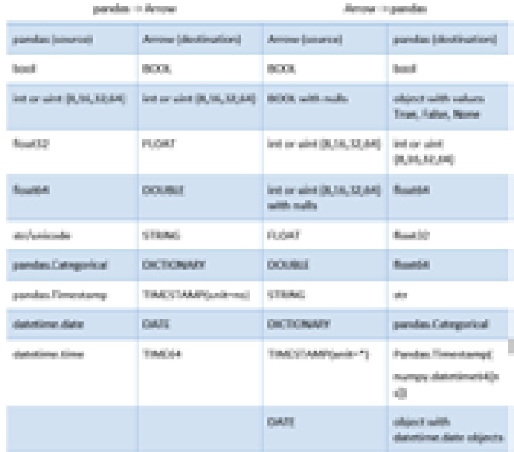
Figure 2.6 – Mapping of pandas types to Arrow types

Only some data types in pandas support handling missing data or null values. A specific case of this is that the default integer types do not support nulls and will get cast to float when converting from Arrow if there are any nulls in the array. If there are no nulls, then the column remains the integer type it had before conversion, as shown in the following snippet:

>>> arr = pa.array([1, 2, 3])

>>> arr

<pyarrow.lib.Int64Array object at 0x000002348DCD02E8>

[

  1,

  2,

  3

]

>>> arr.to_pandas()

0  1

1  2

2  3

dtype: int64

>>> arr = pa.array([1, 2, None])

>>> arr.to_pandas()

0  1.0

1  2.0

2  NaN

dtype: float64

When you're working with date and time types there are a few caveats that need to be kept in mind regarding knowing what data type to expect, as follows:

• Most of the time, dates in pandas are handled using the numpy.datetime64[ns] type, but sometimes, dates are represented using arrays of Python's built-in datetime.date object. Both will convert into the Arrow date32 type by default:
  • If you want to use date64, you must specify it explicitly:

    >>> from datetime import date

    >>> s = pd.Series([date(1987, 8, 4), None, date(2000, 1, 1)])

    >>> arr = pa.array(s)

    >>> arr.type

    DataType(date32[day])

    >>> arr = pa.array(s, type='date64')

    >>> arr.type

    DataType(date64[ms])

  • Converting back into pandas will get you datetime.date objects. Use the date_as_object=False argument to get NumPy's datetime64 type:

    >>> arr.to_pandas()

    0   1987-08-04

    1   None

    2   2000-01-01

    dtype: object

    >>> s2 = pd.Series(arr.to_pandas(date_as_object=False))

    >>> s2.dtype

    dtype('<M8[ns]')

• Python's built-in datetime.time objects will be converted into Arrow's time64 type and vice versa.
• The timestamp type that's used by pandas is NumPy's datetime64[ns] type, which is converted into an Arrow timestamp using nanoseconds as the unit.
  • If you're using a time zone, it will be preserved via metadata when converting. Also, notice that the underlying values are converted into UTC in Arrow, with the time zone in the data type's metadata:

    >>> df = pd.DataFrame({'datetime': pd.date_range('2020-01-01T00:00:00-04:00', freq='H', periods=3)})

    >>> df

                       datetime

    0 2020-01-01 00:00:00-04:00

    1 2020-01-01 01:00:00-04:00

    2 2020-01-01 02:00:00-04:00

    >>> table = pa.Table.from_pandas(df)

    >>> table

    pyarrow.Table

    datetime: timestamp[ns, tz=-4:00]

    datetime: [[2020-01-01 04:00:00.000000000,2020-01-01 05:00:00.000000000,2020-01-01 06:00:00.000000000]]

Since pandas is used so extensively in the Python ecosystem and already provides utilities for reading and writing CSV, Parquet, and other file types, it may not necessarily be clear what advantages Arrow provides here other than interoperability. That's not to say that providing interoperability for pandas with any utility built for Arrow isn't a huge benefit – it is! But this integration shines when you're considering memory usage and the performance of reading, writing, and transferring the data.

Making pandas run fast

With all the optimizations and low-level tweaks that Arrow has to ensure performant memory usage and data transfer, it makes sense for us to compare reading in data files between the Arrow libraries and the pandas library. Using the IPython utility, it's really easy to do timing tests for comparison. We're going to use the same sample data files we did for the examples of reading data files to do the tests:

In [1]: import pyarrow as pa

In [2]: import pyarrow.csv

In [3]: %timeit table = pa.csv.read_csv('train.csv')

177 ms ± 3.03 ms per loop (mean ± std. dev. Of 7 runs, 1 loop each)

The preceding output shows the results of using the timeit utility to read the CSV file in using pyarrow seven times and getting the average and standard deviation of the time each took. On my laptop, it took only 177 milliseconds on average to create an Arrow table from the CSV file, which is around 192 megabytes in size. To keep a fair comparison, we also need to time how long it takes to create the pandas DataFrame from the Arrow table so that we're comparing apples to apples:

In [4]: table = pa.csv.read_csv('train.csv')

In [5]: import pandas as pd

In [6]: %timeit df = table.to_pandas()

509 ms ± 10.7 ms per loop (mean ± std. dev. Of 7 runs, 1 loop each)

At around 509 milliseconds, we see it took much longer to convert the table into a DataFrame than it took to even read the file into the Arrow table. Now, let's see how long it takes to read it in using the pandas read_csv function:

In [7]: %timeit df = pd.read_csv('train.csv')

3.49 s ± 193 ms per loop (mean ± std. dev. Of 7 runs, 1 loop each)

Wow! Look at that! On my laptop, it took an average of 3 and a half seconds to read the file using pandas directly. Even combining the cost of reading the file in and converting it from Arrow into a DataFrame, that's just over an 80% difference in performance with this fairly small (by data analysis standards) file containing 1,458,644 rows and 11 columns. I'll give pandas a fighting chance, though. We can try reading from a compressed version of the CSV file, causing there to be added processing that must be performed to decompress the data before it can be parsed to create the final objects. The following chart contains the final times from using the timeit utility, not just for reading the file and its compressed form, but also for writing the CSV file from the data:

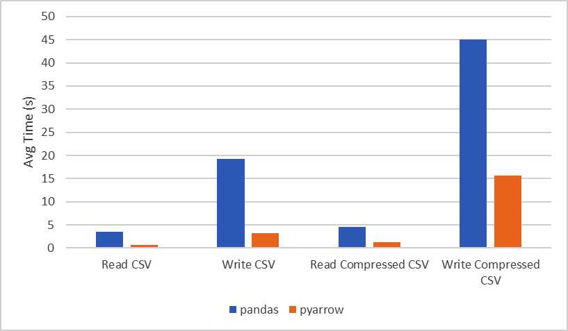
Figure 2.7 – Runtime comparison for reading and writing a CSV file

You might be wondering about the other file formats besides CSV and how the performance compares between pandas and pyarrow. If you look at the documentation for the functions in pandas that deal with Parquet and ORC file formats, you'll find that in both cases, it just delegates calls out to the pyarrow library and uses it to read the data in. For the JSON use case, the structure and format of the data expected by pandas is different than what is expected by pyarrow, so it's not an equivalent use case. Instead, you should choose based on which conforms to what you need. This usually depends on the source of the data you'll be using.

Occasionally, when you're performing the conversions between Arrow arrays or tables and pandas DataFrames, memory usage and performance issues can rear their ugly heads. Because the internal representation of the raw data is different between the two libraries, there are only a limited number of situations where the conversion can occur without you having to copy data or perform computations. At worst, the conversion can result in having two versions of your data in memory, which is potentially problematic, depending on what you're doing. But don't fret! We're going to cover a few strategies to mitigate this problem next.

Keeping pandas from running wild

In the previous section, we saw it took a little more than 500 ms to create a pandas DataFrame from the Arrow table of our CSV data. If that seemed to be a little slow to you, it's because it had to copy all those strings we have in the data. The functions for converting Arrow tables and arrays into DataFrames have an argument named zero_copy_only that, if set to true, will throw an ArrowException if the conversion requires the data to be copied. It's kind of an all-or-nothing situation that should be reserved for only if you need to micromanage your memory usage. The requirements that need to be met for a zero-copy conversion are as follows:

• Integral (signed or unsigned) data types, regardless of the bit width, or a floating-point data type (float16, float32, or float64). This also covers the various numeric types that are represented using this data, such as timestamps, dates, and so on.
• The Arrow array contains no null values. Arrow data uses bitmaps to represent null values, which pandas doesn't support.
• If it is a chunked array of data, then it needs to be only a single chunk because pandas requires the data to be entirely contiguous.

Two options are provided by the pyarrow library to limit the potential copies of data during conversion – split_blocks and self_destruct. Because pandas uses NumPy under the hood for its computations, it likes to collect columns of the same data type in two-dimensional NumPy arrays because it speeds up the – already very speedy –  operations on many columns at once, such as gathering the sum of multiple columns. The following diagram shows a very simplified visual as to how the memory of a DataFrame is managed in pandas. There's an object called a Block Manager that handles memory allocations and keeps track of where the underlying arrays of data are. Unfortunately, if you are gradually building up a DataFrame column by column every so often, the Block Manager is going to consolidate those individual columns into groups called blocks, and that consolidation will require copying the data internally to put the block together:

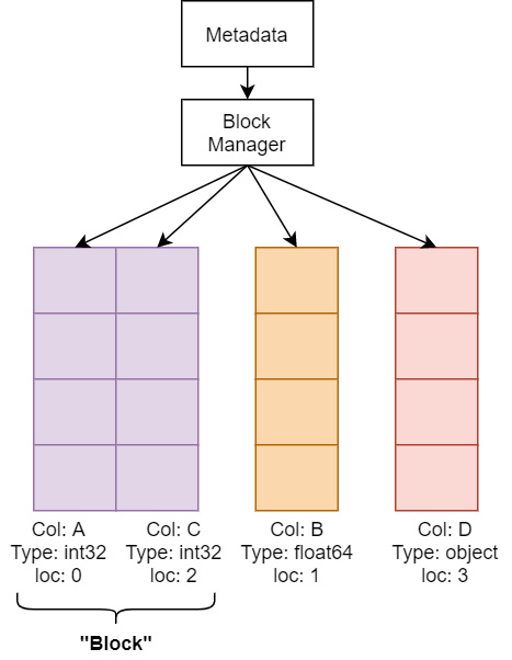
Figure 2.8 – Simplified DataFrame memory layout

The pyarrow library tries very hard to construct the exact consolidated blocks that would be expected so that pandas won't perform extra allocations or copies after converting them into a DataFrame. The downside to doing this is that it requires copying the data from Arrow, which means your peak memory usage would be double the full size of your data. The previously mentioned split_blocks option for conversion produces a single block for each column instead of performing the consolidation beforehand if set to True. Keep in mind that plenty of pandas operations are going to trigger it to start consolidating internally anyway, but this is going to both speed up the conversion process and potentially avoid the worst-case scenario of completely doubling the memory usage for your data. With this option set, if your data meets the criteria for a zero-copy conversion, you will get a true zero-copy operation.

Let's see this in action:

1. First, we must import the libraries we need – that is, pandas, pyarrow, and numpy:

   import pandas as pd

   import pyarrow as pa

   import numpy as np

2. Then, we must create a whole bunch of random floating-point data to test with as NumPy arrays:

   nrows = 1_000_000

   ncols = 100

   arr = np.random.randn(nrows)

   data = {'f{}'.format(i): arr for i in range(ncols) }

3. Now, we must time our conversions – let's see how it goes:

   In [8]: %timeit df = pd.DataFrame(data)

   157 ms ± 13.6 ms per loop (mean ± std. dev. of 7 runs, 1 loop each)

   In [9]: %timeit df = pa.table(data).to_pandas()

   115 ms ± 4.91 ms per loop (mean ± std. dev. of 7 runs, 10 loops each)

   In [10]: %timeit df = pa.table(data).to_pandas(split_blocks=True)

   3.18 ms ± 37.3 µs per loop (mean ± std. dev. of 7 runs, 100 loops each)

Sorcery! Of course, if you followed these conversions up with a bunch of pandas operations, the 100 milliseconds that you saved on the conversion may instead show up when the next consolidation happens, but the numbers are pretty impressive! Even in the case where Arrow does the consolidation, the conversion was faster than just creating the DataFrame from the NumPy arrays in the first place by around 26%. One of the reasons that Arrow does all this work when constructing DataFrames, and doing it as fast and efficiently as possible, is to prevent everyone from having to come up with converters for DataFrames. Components, utilities, and systems can just produce Arrow formatted data in whatever language they want (even if they don't depend on the Arrow libraries directly!) and then use pyarrow to convert it into a pandas DataFrame. Don't go writing a converter – the Arrow library is likely going to be much faster than any custom conversion code and you will end up with less code to maintain. It's a win-win!

But what about the ominous-sounding self_destruct option? Normally, when you copy the data, you end up with two copies in memory until the variable goes out of scope and the Python garbage collector cleans it up. Using the self_destruct option will blow up the internal Arrow buffers one by one as each column is converted for pandas. This has the potential of releasing the memory back to your operating system as soon as an individual column is converted. The key thing to remember about this is that your Table object will no longer be safe to use after the conversion and trying to call a method on it will crash your Python process. You can also use both options together which will, in some situations, result in significantly lower memory usage:

>>> df = table.to_pandas(split_blocks=True, self_destruct=True)

>>> del table # not necessary but good practice

Note

Using self_destruct is not necessarily guaranteed to save memory! Because the conversion is happening with each column as it is converted, freeing the memory is also happening column by column. In the Arrow libraries, it is possible, and frequently likely, that multiple columns could share the same underlying memory buffer. In this situation, no memory will be freed until all of the columns that reference the same buffer are converted.

We've talked a lot about zero-copy up to this point with it coming up here and there as I've introduced various ways Arrow enables transferring data around. The nature of Arrow's columnar format makes it very easy to stream and shift raw buffers of memory around or repurpose them to increase performance. Usually, when data is being passed around, there is a need to serialize and deserialize information, but you'll remember that previously, I said that Arrow allows you to skip the serialization and deserialization costs.

To ensure efficient memory usage when you're dealing with all these streams and files, the Arrow libraries all provide various utilities for memory management that are also utilized internally by them. These helper classes and utilities are what we're going to cover next so that you know how to take advantage of them to make your scripts and programs as lean as possible. We're also going to cover how you can share your buffers across programming language boundaries for improved performance, and why you'd want to do so.

Sharing is caring… especially when it's your memory

Earlier, we touched on the concept of slicing Arrow arrays and how they allow you to grab views of tables or record batches or arrays without having to copy the data itself. This is true down to the underlying buffer objects that are used by the Arrow libraries, which can then be used by consumers, even when they aren't working with Arrow data directly to manage their memory efficiently. The various Arrow libraries generally provide memory pool objects to control how memory is allocated and track how much has been allocated by the Arrow library. These memory pools are then utilized by data buffers and everything else within the Arrow libraries.

Diving into memory management

Continuing with our examination of the Go, Python, and C++ implementations of Arrow, they all have similar approaches to providing memory pools for managing and tracking your memory usage. The following is a simplified diagram of a memory pool:

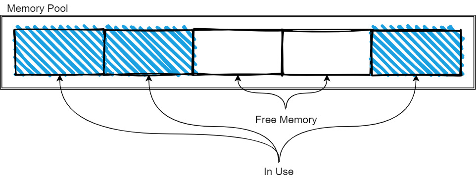
Figure 2.9 – Memory pool tracking memory

As more memory is needed, the pool is expanded as it allocates more memory. When memory is freed, it is released back to the pool so that it can be reused by future allocations. The exact management strategy will vary from implementation to implementation, but the basic idea is still like what's shown in the preceding diagram. The memory pools are typically used for the longer-lived and larger-sized data, such as the data buffers for arrays and tables, whereas the small, temporary objects and workspaces will use the regular allocators for whatever programming language you're working in.

In most cases, a default memory pool or allocator will be used (which you can see in several of the previous code examples), but many of the APIs allow you to pass in a specific memory pool instance to perform allocations with, as follows:

C++

The arrow::MemoryPool class is provided by the library for manipulating or checking the allocation of memory. A process-wide default memory pool will be initialized when the library is first initialized. This can be accessed in code via the arrow::default_memory_pool function. Depending on how the library was compiled and the ARROW_DEFAULT_MEMORY_POOL environment variable, the default pool will either be implemented using the jemalloc library, the mimalloc library, or the standard C malloc functions. The memory pool itself has functions to manually release unused data back to the operating system (best effort and only if the underlying allocator holds onto unused memory), to report the peak amount of memory allocation for the pool, and to return the current number of bytes allocated but haven't been freed through the pool.

Memory Allocators

The benefit of using custom allocators such as jemalloc or mimalloc is the potential for significant performance improvements. Depending on the benchmark, both have shown lower system memory usage and faster allocations than the old standby of malloc. It's worth testing your workloads with different allocators to see if you may benefit from them!

For manipulating buffers of data, there is the arrow::Buffer class. Buffers can be pre-allocated, similar to using STL containers such as std::vector via the Resize and Reserve methods by using a BufferBuilder object. These buffers will either be marked as mutable or not based on how they were constructed, indicating whether or not they can be resized and/or reallocated. If you're using I/O functionality such as an InputStream object, it's recommended to use the provided Read functions to read into a Buffer instance because in many cases, it will be able to slice the internal buffer and avoid copying additional data. The following diagram shows an allocated buffer with a length and capacity, along with a sliced view of the buffer. The slice knows that it does not own the memory it points to, so when it is cleaned up, it won't attempt to free the memory:

Figure 2.10 – Mutable buffer and slice

Python

Because the Python library is built on top of the C++ library, all of the functionality mentioned previously regarding memory pools and buffers is also available in the Python library. The pyarrow.Buffer object wraps the C++ buffer type to allow the other, higher-level classes to interact with memory that they may or may not own. Buffers can create parent-child relationships with other buffers by referencing each other via slices and memory views, so that memory can be easily shared across different arrays, tables, and record batches instead of copied. Anywhere that a Python buffer or memory view is required, a buffer can be used without you having to copy the data:

>>> import pyarrow as pa

>>> data = b'helloworld'

>>> buf = pa.py_buffer(data)

>>> buf

<pyarrow.lib.Buffer object at 0x000001CB922CA1B0>

No memory is allocated when calling the py_buffer function. It's just a zero-copy view of the memory that Python already allocated for the data bytes object. If a Python buffer or memory view is required, then a zero-copy conversion can be done with the buffer:

>>> memoryview(buf)

<memory at 0x000001CBA8FECE88>

Lastly, there's a to_pybytes method on buffers that will create a new Python bytestring object. This will make a copy of the data that is referenced by the buffer, ensuring a clean break between the new Python object and the buffer.

Once again, since everything is backed by the C++ library, the Python library has its own default memory pool that can tell you how much data has been allocated so far. We can allocate our own buffer and see this happen:

>>> pa.total_allocated_bytes()

0

>>> buf = pa.allocate_buffer(1024, resizable=True)

>>> pa.total_allocated_bytes()

1024

>>> buf.resize(2048)

>>> pa.total_allocated_bytes()

2048

>>> buf = None

>>> pa.total_allocated_bytes()

0

You can also see that once the memory has been garbage collected, it is freed and the memory pool reflects that it's no longer allocated.

Golang

As with the Python and C++ libraries, the Go library also provides buffers and memory allocation management with the memory package. There is a default allocator that exists that can be referenced by memory.DefaultAllocator, which is an instance of memory.GoAllocator. Because the allocator definition is an interface, custom allocators would be easy to build if desired for given projects. If the C++ library is available, the "ccalloc" build tag can be provided when you're building a project using the Go Arrow library. Here, you can use CGO to provide a function, NewCgoArrowAllocator, which creates an allocator that allocates memory using the C++ memory pool objects rather than the default Go allocators. This is important to utilize if you need to pass memory back and forth between Go and other languages to ensure that the Go garbage collector doesn't interfere.

Finally, there is the memory.Buffer type, which is the primary unit of memory management in the Go library. It works similarly to the buffers in the C++ and Python libraries, providing access to the underlying bytes, being potentially resizable, and checking their length and capacity when wrapping slices of bytes.

Managing buffers for performance

With this memory and buffer management, we can imagine a couple of scenarios where this can all come together to ensure superior performance, as follows:

• Suppose you want to perform some analysis on a very large set of data with billions of rows. A common way to improve this performance would be to parallelize the operations on subsets of rows. By being able to slice the arrays and data buffers without having to copy the underlying data, this parallelization becomes faster and has lower memory requirements. Each batch you operate on isn't a copy – it's just a view of the data, as shown in the following diagram. The dotted lines on the sliced columns indicate that they are just views over a subset of the data in their respective column, in the same way that the preceding diagram demonstrates a sliced buffer. Each slice can be safely operated on in parallel:

Figure 2.11 – Slicing a table without copying

• Maybe you have a series of columns of data and you want to incrementally filter out rows where every column is null. The naive approach would be to simply iterate the rows and copy the data to a new version of each column if at least one of them is not null at that index. This could become even more complex if you're dealing with nested columns. Instead, when using Arrow arrays, you could use the validity bitmap buffers to speed this up! Just perform a bit-wise or operation with all the bitmaps to get a single bitmap that represents the final filtered indexes. Then, rather than having to progressively build up a filtered copy of every single column, you could do it column by column to achieve better CPU cache hits and memory locality. The following diagram shows this process visually. Depending on the total size of the data and the number of rows in the result, it may make more sense to just take slices of each group of rows instead of copying them to new columns. Either way, you are in control of how and when the memory is used and freed:

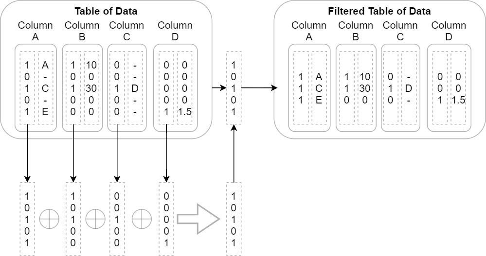
Figure 2.12 – Optimized table filter process

If you're able to pass the address of some buffer of data around, and you know that Arrow's memory format is language agnostic, that means that with just a bit of metadata, you can even share tables of data between different runtimes and languages. Why would you want to do that? I hear you ask. Well, let's see how that could be useful…

Crossing the boundaries

One of the more common workflows when it comes to data science can be seen in the following diagram:

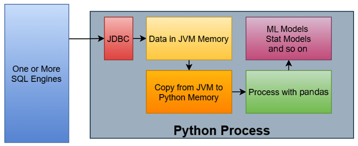
Figure 2.13 – Example data science workflow

The steps of this workflow are as follows:

1. Data is queried from one or more SQL engines from a Python process using a JDBC driver via some library.
2. The rows of data, now residing in JVM memory, are copied into Python memory.
3. The data, now in Python memory, is then processed in some way with pandas.
4. The results of the analysis with pandas are fed into the various models being utilized, such as a machine learning model or some other statistical model.

For large datasets, the most expensive part of this workflow is copying the data from the JVM to Python memory and converting the orientation in pandas from rows into columns. To improve workflows like this, the Arrow libraries provide a stable C data interface that allows you to share data across these boundaries without copying it by directly sharing pointers to the memory. Here, the data is located rather than you creating a huge number of intermediate Python objects. The interface is defined by a couple of header files that are simple enough that they can be copied into any project that is capable of communicating with C APIs, such as by using foreign function interfaces, or FFIs.

In this particular workflow, there is also a JDBC adapter for Arrow in the Java library that retrieves the results, converts the rows into columns in the JVM, and stores data as Arrow record batches in off-heap memory, which is not managed by the JVM itself. This native memory layout can then use the C data interface to inform the pyarrow library of pointers to the raw data buffers and logical structure so that the library can interpret the memory in place properly and use it. The following diagram shows the new workflow using these interfaces:

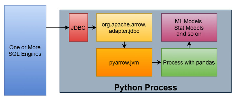
Figure 2.14 – Example data science workflow with memory sharing

This time, the workflow is like this:

1. Data is queried from one or more SQL engines from a Python process using a JDBC driver via some library.
2. As the rows of data come in, they are converted into columnar formatted Arrow record batches with the raw data stored "off-heap" and not managed by the JVM.
3. Instead of copying the data, the Arrow data is accessed directly in Python via the pointers to the data that have already been allocated by the JVM. No intermediate Python objects are created and no copies are made of the raw data.
4. We can now perform the conversion into pandas DataFrames, as we've seen previously, on the Arrow record batches.
5. Finally, those DataFrames are passed to the desired libraries to populate models with the analyzed data.

This may not seem like a lot, but in practice, it can result in humongous performance speedups. Utilizing Dremio as the SQL engine and the sample NYC Taxi dataset, I compared the performance of the two approaches:

• With the former approach, a fairly simple query on the dataset that pulls ~623k rows and 6 columns from Dremio and creates a DataFrame from it took, on average, 1 minute and 5 seconds.
• With the latter approach, while sharing the memory to avoid the copies, the same query took around 573 milliseconds. That's about 113 times faster or an 11,243.8% improvement.

If your result set is small enough, then the benefit of the shared memory approach won't be as large and may not be worth the extra complexity and dependency. The following table shows the performance of the two approaches with different numbers of rows, all at 6 columns each. We can see that if you've got around less than 10,000 rows, even if the relative numbers show significant speedups, the absolute amount of time isn't that much, depending on your workflow:

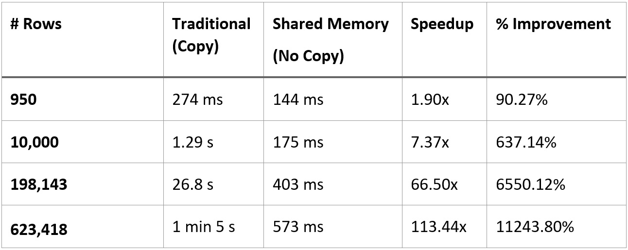
Figure 2.15 – Performance comparison of traditional versus shared memory

Just out of pure curiosity, I tested both workflows with the full dataset in the Parquet file I was using, which comes out to a bit more than 62 million rows of data. The workflow that performs the copying wound up taking a little over 3 hours; utilizing the shared memory utilities across the C data interface only took around 58.7 seconds. This is an astounding ~184 times speedup or ~18,520% improvement!

If you haven't guessed yet, the primary target audience for the C data interface is those developers building libraries, tools, and utilities that use Arrow. Several packages exist already that take advantage of these interfaces, such as the reticulate methods of the arrow R package (https://rstudio.github.io/reticulate/articles/python_packages.html) for passing data between R and Python in the same process and the pyarrow.jvm module I used previously. As more developers and library builders take advantage of the C data interface for passing data around via sharing memory, we'll see the overall performance of common data tasks rocket into the stratosphere, leaving more CPU cycles and memory to be used for performing the necessary analytics computations, rather than on copying data over and over just to make it accessible in the tools you want to use.

If you are one of those library and utility developers or are an engineer working on passing data for other purposes, take advantage and play around with the interface. In addition to the raw data, there is also support for streaming data via the C interface so that you can stream record batches directly into shared memory instead of copying them. At the time of writing, facilities for using the C data interface exist in the C++, Python, R, Rust, Go, Java, C/GLib, and Ruby implementations of the Arrow library. Go take advantage of this awesome way to share data between tools! Go!

Summary

At this point, not only should you be fairly well acquainted with a variety of topics and concepts regarding the usage of the Apache Arrow libraries, but you should also know how to start integrating them into your daily workflows. Whether you're taking advantage of the filesystem abstractions, data format conversions, or zero-copy communication benefits, Arrow can slot into a huge number of parts of any data workflow. Make sure you understand the concepts that have been touched on so far involving the formats, communication methods, and utilities provided by the Arrow libraries before moving on. Play around with them and try out different strategies for managing your data and passing it around between tools and utilities. If you're an engineer building out distributed systems, try using the Arrow IPC format (which we will learn about in detail in Chapter 4, Format and Memory Handling) and compare that with whatever previous way you passed data around. Which is easier to use? Which is more performant?

The next chapter, Data Science with Arrow, kind of wraps up the first big part of this book by diving more into specific examples of where and how Arrow can enable and enhance data science workflows, as we saw with the memory sharing through the C data interface, which provides huge performance improvements to a fairly standard workflow. We're going to address using ODBC/JDBC more directly, using Apache Spark and Jupyter, and even strategies and utilities for using Elasticsearch and providing interactive charts and tables powered by Arrow.

Ready? Let's do this!