1
From the Calculator to the Supercomputer
1.1. Introduction
As noted in the Preface of this book, almost everyone uses computers, often unknowingly, in both professional and personal activities. The first computers weighed tons and took up a lot of space, while consuming a lot of energy. Today, our mobile phones have several tiny, energy-efficient computers built into them.
The history of these machines, known to us as computers, is marked by a few major steps that we present in this chapter. Let us first look at the evolution of hardware; we will deal with computer networks and software in the chapters that follow.
1.2. Some important concepts
Before describing the main steps that precede the construction of the first computers, let us clarify a few concepts that are important in this history.
1.2.1. Information and data
The word “information” covers a wide variety of fields. For example, our five senses (sight, smell, taste, hearing and touch) transmit information to our brains that is essential to our lives and even our survival.
Native Americans exchanged more structured information (e.g. as a way of inviting people to a tribal gathering) by means of smoke signals. These signals were coded and communicated, but they could not be stored.
Today, the word “information” is predominantly used to refer to events such as those presented in journalism (written or digital press, television news, radio, etc.). For our purposes, we will use a narrower definition: information is an element of knowledge that can be translated into a set of signals, according to a determined code, in order to be stored, processed or communicated.
Analog information is supported by a continuous signal, an oscillation in a power line, for example, or a bird song. Digital information is information that is symbolically coded with numbers (e.g. 384,400 for the distance in kilometers from the Earth to the Moon).
The theoretical concept of information was introduced from theoretical research on electrical communication systems. In a general sense, an information theory is a theory that aims to quantify and qualify the notion of information content present in a dataset. In 1948, the American mathematician Claude Shannon published the article, “A Mathematical Theory of Communication”1 and has since been considered the father of information theory.
Data are what computers deal with, and we will come back to data in Chapter 4. These are raw quantities (numbers, texts, etc.) that will be digitized (converted into a series of numbers) so that they can be understood and manipulated by computers. Alphabetic characters (and other characters) can be easily digitized. A sound can be represented by a sequence of regularly sampled sound intensities, each digitally encoded. The information contained in digital data, that is, a number, depending on its context (on a pay slip, name and gross salary is information obtained from digital data based on their place on the pay slip).
1.2.2. Binary system
Computers process digital data encoded in base-2, and we will see why; but first, a brief description of this binary system.
We usually count in base-10, the decimal system that uses 10 digits (0, 1, 2, 3, 4, 5, 6, 7, 8, 9). To go beyond 9, we have to “change rank”: if the rank of the units is full, we start the rank of the tens and reset the units to zero and so on. So, after 9, we have 10. When you get to 19, the row of units is full. So, we add a dozen and reset the unit rank to zero: we get to 20.
The binary system, or base-2 numbering system, uses only two symbols, typically “0” and “1”. The number zero is written as “0”, one is written as “1”, two is written as “10”, three is written as “11”, four is written as “100”, etc. In the binary system, the unit of information is called the bit (contraction of “binary digit”). For example, the base-2 number “10011” uses 5 bits.
It is quite easy to convert a decimal number (dn) to a binary number (bn). The simple solution is to divide the dn by 2; note the remainder of the division (0 or 1) which will be the last bit of the bn, start again with the previous quotient until the quotient is zero. For example, if the dn is 41, the division by 2 gives 20 + 1; the last bit (called rank 1) of the bn is 1; we divide 20 by 2, which gives 10 + 0; the bit of rank 2 is 0; we divide 10 by 2, which gives 5 + 0; the bit of rank 3 is 0; we divide 5 by 2, which gives 2 + 1; the bit of rank 4 is 1; we divide 2 by 2, which gives 1 + 0; the bit of rank 5 is 0; we divide 1 by 2, which gives 0 + 1; the bit of rank 6 is 1. So, the binary number is 101001.
The importance of the binary system for mathematics and logic was first understood by the German mathematician and philosopher Leibnitz in the 17th century. The binary system is at the heart of modern computing and electronics (calculators, computers, etc.) because the two numbers 0 and 1 are easily translated into the voltage or current flow.
1.2.3. Coding
In real life, the same information can be represented in different ways. For example, administrations use different forms to represent a date of birth: January 10, 1989; 01/10/1989; 10/JAN/89; etc. It is therefore necessary to agree on the same way of representing numbers and characters. This is coding.
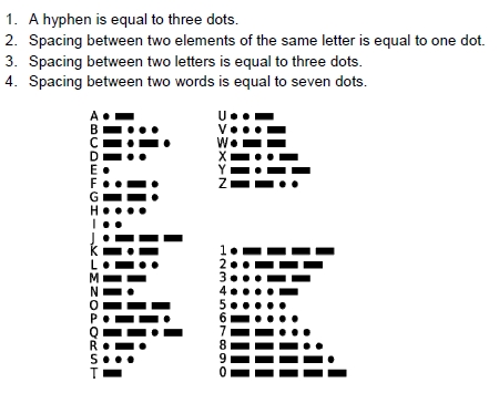
Coding of information has existed for several years. For example, Morse code, named after its inventor Samuel Morse (1791–1872), is a telegraphic code using a conventional alphabet to transmit a text, using a series of long and short pulses.
Information coding refers to the means of formalizing information so that it can be manipulated, stored or transmitted. It is not concerned with the content but only with the form and size of the information to be coded.
With the advent of the computer, it has been necessary to develop data coding standards to facilitate their manipulation by computer tools around the world. We can represent the set of characters by binary codes of determined length. Binary is used for obvious reasons, one bit being the minimum amount of information that can be transmitted.
In computer science, we mainly use the bit, the byte (unit of information composed of 8 bits, which allows us to store a character such as a number or a letter) and the word (unit of information composed of 16 bits). We commonly use multiples: kilobyte (KB) for a thousand bytes, megabyte (MB) for a million bytes, gigabyte (GB) for a billion bytes and so on.
1.2.4. Algorithm
What should the computer do with this data encoded in binary numbers? What processing must it do? Adding two numbers is a trivial process, but we expect much more from a computer, and we must tell it what is expected of it!
The word algorithm comes from the name of the great Persian mathematician Al Khwarizmi (ca. 820 CE), who introduced decimal numeration (brought from India) in the West and taught the elementary rules of calculation related to it. The notion of the algorithm is thus historically linked to numerical manipulations, but it has gradually developed to deal with increasingly complex objects, texts, images, logical formulas, etc.
An algorithm, very simply, is a method, a systematic way of doing something: sorting objects, indicating a path to a lost tourist, multiplying two numbers or looking up a word in the dictionary. A recipe can be considered an algorithm if we can reduce its specificity to its constituent elements:
- – input information (ingredients, materials used);
- – simple elementary instructions (slicing, salting, frying, etc.), which are carried out in a precise order to achieve the desired result;
- – a result: the prepared dish.
Algorithms, in the computer sense, appeared with the invention of the first machines equipped with automations. More precisely, in computer science, an algorithm is a finite and unambiguous sequence of operations or instructions to solve a problem or to obtain a result. It can be translated, thanks to a programming language, into a program executable by a computer.
Here is a simple example, the algorithm for determining the greatest common divisor (GCD) of two integers, a and b (Euclid’s algorithm):
READ a and b
If b>a, then PERMUTE a and b
RETURN
r=the remainder of the division of a by b
If r is different from 0
  REPLACE a by b then b by r
  GO TO RETURN
WRITE b
END
Algorithms, in the real lives of computer scientists, are of course more complex. We have therefore tried to represent them in a more readable way and, above all, without any ambiguity, always possible in the interpretation of a text. Programming flowcharts are a standardized graphical representation of the sequence of operations and decisions carried out by a computer program. Figure 1.2 shows a flowchart of the Euclidean algorithm.
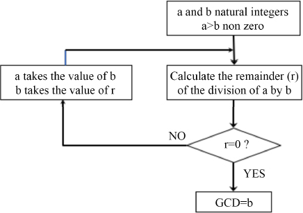
Figure 1.2. Flowchart of the Euclidean algorithm
We can usually solve a problem in several ways, and thus can write different algorithms, but all should lead to the same result. The algorithm’s quality will be measured by criteria such as efficiency (speed of obtaining the result), the quantity of resources consumed, the accuracy of the result obtained, etc.
1.2.5. Program
An algorithm can be translated, using a programming language, into a sequence of instructions or a program that can be executed by a computer. For human beings, writing sequences of 0 and 1 is not much fun, not very readable, and can lead to many errors. We have therefore invented increasingly advanced programming languages, some quite general, others more adapted to specific fields. The program, written in such a language, will be translated by a program called a compiler in the language known by the machine.
A program represents an algorithm. It is a sequence of instructions defined in a given language and intended to be executed by a computer. This language has, like any language, its alphabet, its words, its grammar and its rules. We will come back to programs and programming languages in Chapter 3.
1.3. Towards automation of calculations
For millennia, humans have used their fingers, stones or sticks to calculate. Then, more sophisticated tools appeared: the use of counting frames (trays on which stones or tokens are moved) or the abacus (Middle East, Russia and China).
Numerous scientific contributions, in particular mathematical and technical, have made it possible to build and use machines designed to calculate more easily, more quickly and, in general, reducing the risk of error. These machines became computers, able to solve very different problems, from network gaming to virtual reality and databases.
Here are a few steps that have marked the progression towards certain automation of calculations and tasks to be performed in different contexts.
1.3.1. Slide rule
William Oughtred (1574–1660) developed a slide rule which – by simple longitudinal displacement of graduated scales according to the property of logarithmic functions – enabled the transformation of a product into a sum and a division into a difference, to directly perform arithmetic operations of multiplication and division, and which can also be used to perform more complex operations such as the calculation of square roots, cubic, logarithmic or trigonometric calculations.
Its reign lasted until the mid-1980s, and it was used by many students and engineers until the appearance of pocket calculators.

Figure 1.3. A slide rule (source: Roger McLassus). For a color version of this figure, see www.iste.co.uk/delhaye/computing.zip
1.3.2. The Pascaline
Due to the increase in trade and commerce, people needed more efficient tools to facilitate and, above all, speed up calculations related to commercial transactions. The road to automation was open, and calculators that could progressively automate arithmetic operations were developed.

Figure 1.4. A Pascaline (source: David Monniaux). For a color version of this figure, see www.iste.co.uk/delhaye/computing.zip
In 1642, Blaise Pascal (1623–1662) made the first calculator that allowed additions and subtractions to be made by a system of toothed wheels (a gear made it possible to make a deduction). It was perfected by Leibnitz (1694), who afforded it the ability to carry out multiplications and divisions (by successive additions or subtractions).
The Pascaline was at the origin of many machines, as well as key inventions of the industry.
1.3.3. The Jacquard loom
While, for centuries, human beings have had the ambition to calculate and then to automate calculations, at the dawn of the Industrial Revolution of the 19th century, they also had the ambition to automate tasks. Falcon (a weaver mechanic) used punched cards in the loom around 1750. But Jacquard (1752–1834) industrialized the invention in 1781. In an endless movement, a series of punched cards attached to each other were passed in front of needles and thus allowed a precise weaving. The punched cards guided the hooks that lift the warp threads, thus enabling complex patterns to be woven. This is an early application of the aforementioned concept of the program. Simple to install, the Jacquard loom spread rapidly throughout Europe. In Lyon, the Jacquard loom was not well received by silk workers (the Canuts) who saw it as a possible cause of unemployment. This led to the Canuts’ revolt, during which the workers destroyed machines.
1.3.4. Babbage’s machine
In 1833, the British mathematician Charles Babbage (1791–1871), who was passionate about Jacquard’s work, proposed a very advanced mechanical calculator: the analytical machine. It was a programmable mechanical calculator that used punched cards for its data and instructions, but the machine was never completed. Mathematician Ada Lovelace2, colleague of Charles Babbage, designed a series of programs (sequences of punched cards) for this machine.
1.3.5. The first desktop calculators
The German mathematician Gottfried von Leibnitz (1646–1716) built a more sophisticated machine than the Pascaline, without any real success. Based on this model, in 1820 the Frenchman Thomas de Colmar (1785–1870) invented the arithmometer, a practical, portable and easy-to-use machine. It was an entirely mechanical calculator capable of performing the four operations of arithmetic (addition, subtraction, multiplication and division). It was the first calculator produced in series and marketed (between 1851 and 1915) with great success (more than 1,500 calculators were sold in France).
At the end of the 19th and beginning of the 20th century, there was an explosion of innovations in office machines, all of which were aimed at making them easier to use thanks to an increase in the proportion of automated systems.
The Curta mechanical calculator, invented by the Austrian engineer Curt Herzstark, was produced between 1948 and 1972. Composed of a cylindrical body and a small crank handle, making it look like a pepper mill, it weighed barely 230 grams. It enables the four basic arithmetic operations to be performed very quickly and, after training, other operations such as square roots. My father, who was an astronomer, used a Curta calculator that I could play with!
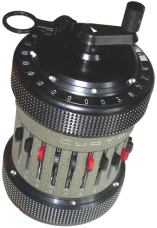
Figure 1.5. The Curta mechanical calculator (source: Jean-Marie Hardy). For a color version of this figure, see www.iste.co.uk/delhaye/computing.zip
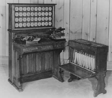
1.3.6. Hollerith’s machine
In response to a competition launched by the US Census Bureau, Hermann Hollerith (1860–1929) built a punch-card statistical machine that uses cards (12 × 6 cm) with the 210 boxes needed to receive the characteristics of an individual: age, sex, occupation, family situation, etc. The machine was designed to be used for the purpose of collecting data on the characteristics of individuals. The cards are read by an electric reader; a hole lets the current pass through and the absence of a hole stops it.
Not only did Hollerith propose to collect the census data of each inhabitant in this form, but, in addition, he designed a machine that allowed for the automatic processing of these punched cards, the machine adding these data together to produce statistics. The 1880 census was processed (manually) in eight years. The census of 1890 was processed in record speed for the time (between six months and a little more than a year, according to sources).
Hollerith left the administration and founded the Tabulating Machine Company in 1896 (later, the Computing-Tabulating-Recording Company, CTR), with Thomas J. Watson as director in 1914. In 1924, the company became International Business Machines Corporation, better known as IBM.
In 1924, Fredrik Bull, a Norwegian engineer, filed a patent on a system similar to the Hollerith system. His patents were sold to the French company, Compagnie des Machines Bull, founded in 1930 for the purpose of exploiting these patents.
1.4. The first programmable computers
How can we avoid turning the crank handle, as we had to do with the Curta machine, to make a calculation? It is the machine itself that will carry out this task thanks to a program, after providing it with the data to be processed. Let us discuss the programmable calculator.
In 1854, George Boole (1815–1864) designed the algebra that bears his name and is based on two signs (YES = 1, NO = 0) and three operators (AND, OR, NOT). Boole’s algebra came to find many applications in computer science and in the design of electronic circuits.
In 1936, Alan Turing3 proposed his definition of a machine, a major contribution to theoretical computer science. He described an abstract machine to give formal support to the notions of algorithm and effective computation.
Electronic circuits, vacuum tubes, capacitors and electronic relays replaced their mechanical equivalents, and numerical computation (using numbers or numerical symbols) replaced analog calculation (using continuous physical measurements, of mechanical or electrical origin) to model a problem. Below are three examples.
1.4.1. Konrad Zuse’s machines
Konrad Zuse (1910–1995) was a German engineer who was one of the pioneers of programmable calculation, which prefigured computer science. He built several machines, but his greatest achievement was the creation of the first programmable binary floating-point electromechanical calculator, the Z3. Started in 1937, it was completed in 1941; it consisted of 2,000 electromechanical relays.
1.4.2. Colossus
Colossus was the first electronic calculator based on the binary system. It was developed in London during World War II (1943). It was a calculator specialized for decrypting the Lorenz code, a secret code the Germans reserved for highly important communications during the war. Colossus, an electronic machine programmable using a wiring board, was made up first of 1,500 and then of 2,400 vacuum tubes and performed 5,000 operations per second.
1.4.3. ENIAC
The first known programmable electronic digital computer, the ENIAC (Electronic Numerical Integrator and Computer) was developed during World War II at the University of Pennsylvania by Americans John P. Eckert and John W. Mauchly. It went into operation in 1946.
Physically, the ENIAC was a big machine: it contained 17,468 vacuum tubes, 7,200 crystal diodes, 1,500 relays, 70,000 resistors, 10,000 capacitors and about 5 million hand-made welds. It weighed 30 tons, occupying an area of 167 m2! ENIAC suffered from the unreliability of its components, which comes as no surprise.
ENIAC made its calculations in the decimal system and could be reprogrammed to solve, in principle, all computational problems.
Programming the ENIAC consisted of wiring connections and adjusting electrical buttons, long and complex operations. It became clear that if it was to be used as a flexible machine, capable of a wide variety of calculations, another form of programming was needed.
1.5. Generations of computers
The automation of calculations was therefore progressing well, but the programming of these machines remained a real problem to which a solution needed to be found. This was the arrival of the first computers, whose program can be stored in the memory of the machine itself. And the evolution of computers has proven spectacular.
The first computers date back to 1949. It was the idea, in 1945, of a recorded program, from the Hungarian–American mathematician and physicist John von Neumann4 and his collaborators, which transformed a calculator into a computer using a unique storage structure to store both the instructions and the data requested or produced by the calculation.
Von Neumann’s architecture breaks down the computer into four distinct parts:
- – a calculating organ, capable of executing arithmetic and logical operations, the arithmetic and logic unit;
- – a central memory, used both to hold the programs describing how to arrive at the results and the data to be processed;
- – input–output organs serving as organs of communication with the environment and with the human;
- – a control unit to ensure consistent operation of the above elements.
The first innovation is the separation between the control unit, which organizes the instruction sequencing flow, and the arithmetic and logic unit, in charge of the execution of these instructions. The second fundamental innovation was the idea of the stored program: instead of being encoded on an external support (tape, cards, wiring board), the instructions are stored in the memory.
A memory location can contain both instructions and data, and a major consequence is that a program can be treated as data by other programs.

The unit formed by the arithmetic and logic unit, on the one hand, and the control unit, on the other hand, constitutes the Central Processing Unit (CPU) or processor. The processor executes the programs loaded into the central memory by extracting their instructions one after the other, analyzing and executing them. All of the physical components, known as hardware, are controlled by software.
Computer calculations are cadenced by a clock whose frequency is measured in hertz. The higher the frequency (and therefore the shorter the basic cycle time), the more operations the computer will be able to perform per second.
The architecture (organization) of computers has evolved and become more complex over the years. Generations of computers are distinguished by the technologies used in the physical components and by the evolution of the software, in particular the operating system, which is the set of programs controlling the various components (processor, memory, peripheral units, etc.) of the computer, thus allowing it to function. The evolution of software is discussed in Chapter 3.
1.5.1. First generation: the transition to electronics
From 1948 onwards, the first von Neumann architecture machines appeared: unlike all previous machines, programs were stored in the same memory as data and could therefore be manipulated as data. This is what the aforementioned compiler does: transforms a program describing an algorithm into a machine-readable program.
The first generation is that of electronic tube machines and electromechanical relays.
1.5.1.1. EDVAC (Electronic Discrete Variable Automatic Computer)
The design of a new machine, more flexible and, above all, more easily programmable than the ENIAC, had already begun in 1944, before the ENIAC was operational. The design of the EDVAC, to which von Neumann made a major contribution, attempted to solve some of the problems posed by ENIAC’s architecture. Like ENIAC, EDVAC was designed by the University of Pennsylvania to meet the needs of the US Army Ballistics Research Laboratory.
The computer was built to operate in binary with automatic addition, subtraction and multiplication, and programmable division, all with automated control and a memory capacity of 1,000 words of 44 bits. It had nearly 6,000 vacuum tubes and 12,000 diodes, consumed 56 kW, occupied an area of 45.5 m2 and weighed 7,850 kg. It calculated 350 multiplications per second and was released in 1949.
Its plans, which were widely disseminated, gave rise to several other computer projects in the late 1940s and up to 1953.
1.5.1.2. Harvard Mark III (1949) and IV (1952)
Designed by Howard H. Aiken (Harvard University), the Harvard Mark III and IV models are among the first registered-program computers. The Mark III, partly electronic and partly electromechanical, was delivered to the US Navy in 1950. The Mark IV, one of the first fully electronic computers, was designed for the Air Force and delivered in 1952.
1.5.1.3. UNIVAC I (Universal Automatic Computer I)
The UNIVAC I was the first commercial computer made in the United States. It used 5,200 vacuum tubes, weighed 13 tons, consumed 125 kW for a computing power of 1,905 operations per second with a 2.25 MHz clock. The first computer equipped with magnetic tape units was manufactured by Univac, a subsidiary of the Remington Rand company.
The first copy was completed in 1951, and 46 copies were delivered up to 1958.
1.5.1.4. IBM 701 and IBM 704
IBM (International Business Machines Corporation), created in 1924, came to have an essential place in the IT world for many years to come. It developed in the 1930s thanks to the patents of mechanography on the perforated card invented by Hermann Hollerith.
In April 1952, IBM produced its first scientific computer, the IBM 701, for the American Defense Service. The first machine was installed at the Los Alamos (New Mexico) laboratory for the American thermonuclear bomb project, and had two twins designed for commercial applications: the IBM 702 and the IBM 650, of which about 2,000 units were produced until 1962.
In April 1955, IBM launched the IBM 704, scientific computer (its commercial counterpart was the 705). It used a memory with ferrite cores, much more reliable and faster than cathode ray tubes, of 32,768 words of 36 bits. According to IBM, the 704 could execute 40,000 instructions per second.
The 700 series computers, which used electronic components based on electronic tubes, were replaced by the 7000 series, which used transistors.
1.5.2. Second generation: the era of the transistor
The transistor was invented in 1947 by Americans John Bardeen, William Shockley and Walter Brattain at Bell Laboratories in New Jersey; they were awarded the Nobel Prize in Physics for this invention in 1956. The transistor represented enormous progress in comparison to electronic tubes: it did the same work as the vacuum lamp of the first computers but, at the same time, was much smaller, lighter and more robust; it also consumed less energy.
Moreover, it worked almost instantaneously once powered up, unlike the electronic tubes, which required about 10 seconds of heating, significant power consumption and a high voltage source (several hundred volts).
This invention had a considerable impact on the design and manufacture of computers.
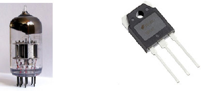
Figure 1.8. An electron tube and a transistor (source: public domain photos)
Transistor-based computers are considered the second generation, and they dominated computing in the late 1950s and early 1960s. Below are a few examples.
1.5.2.1. Bull Gamma 60
In 1958, Compagnie des Machines Bull (France) announced the Gamma 60, delivered in about 15 units from 1960 onwards. This was the first multitasking computer (capable of running several applications simultaneously) and one of the first to feature several processors. It also included several input and output units: magnetic drums, magnetic strips, card readers, card punches, printers, paper strip readers, paper strip punches and a terminal. Its basic cycle time was 10 µs (microseconds). However, the solid-state computer had design flaws typical of an experimental machine.
1.5.2.2. IBM 1401
In 1959, the IBM 1401 appeared, which was the most popular computer system across the world at the beginning of the 1960s. Several factors accounted for this success: it was one of the first computers to operate solely with transistors – instead of vacuum tubes – which made it possible to reduce its size and extend its lifespan; available for rental for $2,500 per month, it was recognized as the first affordable general-purpose computer. Furthermore, the IBM 1401 was also the easiest computer to program at the time.
The 1401 performed 193,000 8-digit additions per minute, and its card reader read 800 cards per minute. It could be equipped with magnetic strips reading an average of 15,000 characters per second. The printer launched with the series produced 600 lines of 132 characters per minute.
Manufactured from 1959 to 1965, it was the best-selling computer of the so-called second-generation computers (more than 10,000 sold).

Figure 1.9. IBM 1401 (source: IBM 1401 Data Processing System Reference Manual)
1.5.2.3. IBM 1620
In 1960, IBM launched the 1620 (scientific) system with different configurations to suit customer needs. There were two models that differed in the cycle time of their memories: 10 µs and 20 µs. Its attractive cost enabled many universities to acquire it, and many students were able to discover computer science thanks to it. About 2,000 units were sold up until 1970.
1.5.2.4. DEC PDP-1
In 1960, Digital Equipment Corporation (DEC) launched the PDP-1 (Programmed Data Processor). The PDP-1 was the first interactive computer (allowing easy exchange between the user and the computer) and introduced the concept of the mini-computer. It had a clock speed of 0.2 MHz (cycle time 5 µs) and could store 4,096 18-bit words. It could perform 100,000 operations per second. Fifty examples were built.
1.5.3. Third generation: the era of integrated circuits
The invention of the transistor quickly called for the development of a technology that would allow the integration of the computer’s different components, because the multiple electrical connections that need to be made between each transistor are complex, expensive to make, not fast enough and not reliable enough.
The first important development with the appearance of the transistor was to mount these transistors on the same circuit board and etch the wires that connected them in the board; the result was known as a printed circuit board. The invention of the printed circuit was attributed to the Frenchman Robert Kapp (1894–1965).
Printed circuits then allowed the invention of the integrated circuit (also called electronic chip), capable of connecting all the elements of the circuit (transistors, diodes, capacitors, wires, etc.) in so-called fully integrated circuits, manufactured in a single operation. The first integrated circuit was invented in 1958 by the American Jack Kilby (1923–2005) while working for Texas Instruments.
Many computers based on these technologies appeared between 1963 and 1971.
1.5.3.1. IBM/360 and IBM/370
The creation of the IBM/360 in 1964 was a turning point in the technical history of computing. Taking advantage of the considerable progress in semiconductor technology, IBM researched and brought to market a range of machines with a large number of innovations. The two lines of IBM production, scientific and commercial, met in the IBM/360 series; the choice of the name 360 reflected the desire to cover the entire horizon of computer applications. The 360 series offered a unique machine architecture, from the smallest (360/20) to the most powerful (360/195), in order to facilitate the changes from one model to a larger one. The smallest computer in the family could make 33,000 additions per second and the largest 2,500,000. The series was equipped with various peripherals, including removable hard disk storage units.
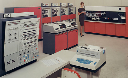
Figure 1.10. IBM/360 computer (source: IBM archives). For a color version of this figure, see www.iste.co.uk/delhaye/computing.zip
The 360 series was followed by the 370 series, announced in 1970. It generalized the virtual memory mechanism and brought significant improvement in processor performance, the basic cycle of the 370/195 being 54 nanoseconds. Marketing of this series was stopped in 1983.
Marketed between 1965 and 1978, for both commercial and scientific applications, more than 14,000 units of this range were sold.
Other manufacturers offered systems compatible with these series, especially Japanese manufacturers (Fujitsu, Hitachi).
IBM dominated the world market by a wide margin in the 1960s, and the reference appeared: “IBM and the 7 dwarves”, when referring to the 7 competitors of the undisputed leader: Burroughs, Univac, NCR, Control Data Corporation, Honeywell, RCA and General Electric.
1.5.3.2. CDC 6600
Control Data occupies a special place in the market of computers dedicated to scientific computing.
Control Data Corporation was a pioneering American company in the manufacture of supercomputers. It was founded in 1957 in Minneapolis-Saint Paul, MN, by American scientists from US Navy research centers, including William Norris and Seymour Cray, who founded Cray Research in 1972. CDC initially focused on computer peripheral units (magnetic tape drives, in particular) before embarking on the construction of computers under the impetus of Seymour Cray.
After the 3600, the first CDC 6600 system was introduced in 1964. At that time, it was 10 times faster than the others. The CDC 6600 was equipped with a transistor CPU with a clock frequency of 10 MHz and had a computing power of 1 Mflops (million floating-point operations per second). This measure of performance in scientific computing was set to continue.
More than 100 units were sold for $8,000,000. This computer is considered to be the first supercomputer ever marketed. It was the most powerful computer between 1964 and 1969 when it was surpassed by its successor, the CDC 7600.
In the late 1970s, Control Data developed the CDC Cyber series, marking a significant improvement in performance, but it was too late to take on the Cray-1, the first supercomputer designed entirely by Seymour Cray.
1.5.3.3. Minicomputers
Until now, computers were mainly developed for and at the request of the military and the major laboratories associated with them. Their cost, both in purchase and in operation, was very high. But the demand from companies and laboratories of all sizes and from the banking sector was pressing: the market for smaller, easier-to-use, less expensive computers pushed manufacturers to diversify their offer.
The minicomputer was an innovation of the 1970s that became significant towards the end of the decade. It brought the computer to smaller or decentralized structures, not only by taking up less space, reducing costs (acquisition and operation) and providing a degree of independence from large IT service providers, but also by expanding the number of computer manufacturers and thus promoting competition. This range of computers has virtually disappeared due to the rise of personal computers.
In the 1980s, Digital Equipment Corporation (DEC) became the second-largest computer manufacturer (after IBM) with its popular PDP computers (especially the PDP-11, DEC’s first machine to use 16-bit rather than 12-bit memory). The PDP series was replaced by the VAX (Virtual Address eXtension), which brought the convenience of the VMS (Virtual Memory System) operating system and was a great success. DEC disappeared in 1998.
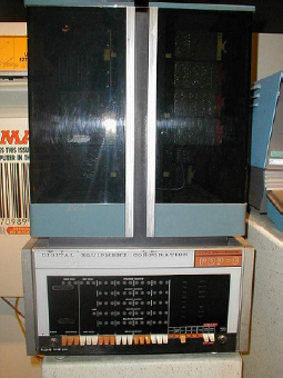
Figure 1.11. A PDP-8 computer (source: Alkivar, Wikipedia). For a color version of this figure, see www.iste.co.uk/delhaye/computing.zip
The Mitra 15 was one of the computers produced by the Compagnie Internationale pour l’Informatique (CII) as part of the Plan Calcul, a French government plan launched in 1966 to ensure the country’s autonomy in information technology. Marketed from 1971 to 1985, it was widely used in higher education and research, as well as for industrial process control and network management. It was also used in secondary education as early as the mid-1970s and was able to operate in conjunction with a large system. A total of more than 7,000 copies were produced.
The Mini 6 was successfully marketed in Europe by the Honeywell-Bull Group from 1976. The Mini 6 was renamed DPS-6 in 1982.
In 1972, Hewlett-Packard launched the HP 3000, a real-time, multi-user, multitasking minicomputer for business applications. At the end of 1980, machines using the HP PA-RISC processor were delivered in large numbers, enabling 32-bit addressing.
In the 1970s, IBM released a series of minicomputers, the 3 series, and then, in the 1980s, the 30 series, which was followed by the AS/400 series that was a great success for management applications (more than 400,000 copies sold).
1.5.4. Fourth generation: the era of microprocessors
One definition, not universally accepted, associates the term “fourth generation” with the invention of the microprocessor.
In 1971, the American company Intel succeeded, for the first time, in placing all the components that make up a processor on a single integrated circuit, thus giving rise to the microprocessor.
The first commercially available (still 4-bit) microprocessor, the Intel 4004, was later expanded to 8 bits under the name Intel 8008. These processors were the precursors of the Intel 8080 and the future Intel x86 processor family.
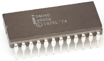
Figure 1.12. Intel 4040 (source: Konstantin Lanzet collection)
Its arrival has led to many advances, such as increased operating speed (distances between components are reduced), increased reliability (less risk of losing connections between components), reduced energy consumption, but above all the development of much smaller computers: microcomputers.
The main characteristics of a microprocessor are:
- – the complexity of its architecture, which is measured by the number of transistors present: the higher the number, the more complex the tasks to be processed can become. Intel’s 4004 included 2,300 transistors; the latest processors include several billions;
- – the speed of its clock that dictates the pace of work; the base frequency of the Intel Xeon Phi KNL processor is 1.30 GHz, while that of the 4004 was 740 kHz (more than 1,000 times slower!);
- – the number of bits it can process (4 at the beginning, 128 in 2011);
- – the fineness of the etching to improve performance and density, and reduce consumption and manufacturing costs.
These characteristics changed very quickly, as shown in Table 1.1, which includes some dates.
Table 1.1. Evolution of Intel processor characteristics (source: Intel)
| Model | Number of transistors | Clock frequency | Fineness of the etching | |
|---|---|---|---|---|
| 1971 | Intel 4004 | 2,300 | 108 kHz | 10 microns |
| 1982 | Intel 286 | 134,000 | 6 MHz | 1.5 micron |
| 1993 | Intel Pentium | 3.1 million | 66 MHz | 0.8 micron |
| 2001 | Intel Xeon | 42 million | 1.7 GHz | 0.18 micron |
| 2008 | Intel Core 2 Duo | 410 million | 2.4 GHz | 45 nm |
| 2012 | 3rd generation Intel Core | 1.4 billion | 2.9 GHz | 22 nm |
In 2019, Intel officially kicked off its generation of 10 nm processors and the stacking of the different layers of the processor in a 3D design. But the improvement of these features may have limits, which I will discuss further with the race for performance.
Manufacturers Intel and AMD dominate the market for microprocessors, which are found in almost all electronic equipment today.
1.5.4.1. The invasion of microprocessors
Today, microprocessors are found in all areas of personal and professional life.
Thanks to tremendous progress in their miniaturization, they are present in our everyday equipment, such as tablets, cell phones, cars, TV sets, game consoles and our bank cards. They are also essential in factories (robots, etc.), in public transportation systems, hospitals, etc.
Some of these areas will be examined in more detail in Chapter 6, on the uses and applications of computer science.
1.5.4.2. The race for performance
Regardless of the equipment considered, the performance of the processor(s) in this equipment is an important factor. If my car’s ABS system responds late, I am at risk of an accident. If the display on my game console is too slow, I am angry.
Co-founder of the Intel company, Gordon Moore stated, as early as 1965, that the number of transistors per circuit of the same size would double, at constant prices, every year (Moore’s law). He later corrected this by increasing the doubling rate to 18 months. He deduced that the power of computers would grow exponentially for years to come. His law, based on an empirical observation, has been verified, even if microprocessor manufacturers now speak of a rate of two years, or even two and a half years.
The increase in performance has therefore been achieved, for a long time, thanks to the evolution of the architecture and the increase in frequency.
Processor architecture has undergone very significant transformations to limit time losses (cycle losses): parallelism in the processors, increase in memory size and hierarchization (e.g. a cache memory integrated in the processor and clocked at the same frequency), etc.
The increase in frequency leads to an increase in the electrical power required, and therefore in the thermal energy generated, which must be dissipated. And the energy consumption of many devices must be controlled, for example, in our smartphones, because it reduces the device’s autonomy.
The solution was first found in 2001 with the first multi-core processor: rather than having a single high-frequency processor, for example, two “cores” with lower frequencies were used, each capable of processing instructions individually. This approach became widespread, and by 2018, the most powerful processors had several dozen cores (64 for the Intel Xeon Phi KNL processor, 260 for the Chinese ShenWei SW26010 processor).
Another approach has been to manufacture specialized microprocessors, that is, adapted to a specific need and stripped of everything that is not necessary for its specified use. We have therefore developed coprocessors, electronic circuits designed to add a function to a conventional processor, graphics processors or GPUs (Graphics Processing Unit), FPGAs (Field-Programmable Gate Array), reprogrammable silicon integrated circuits, etc.
1.5.4.3. Microcomputers
Consumer microcomputers, or personal computers, appeared in the late 1970s, when the size and cost of a computer allowed an individual to acquire his/her own computer.
Apple’s Apple II, Tandy’s TRS-80 and Commodore’s PET were introduced in 1977.
The 1980s saw the multiplication of microcomputers; many American, European and Asian companies rushed into this new market.
The first commercial success was the IBM PC (1981), equipped with an Intel processor, whose descendants and PC-compatible products (often manufactured in Asia) still largely dominate the market. IBM abandoned this niche in the highly competitive microcomputer market in 2005 when it sold its PC division to the Chinese manufacturer Lenovo.
The first Apple Macintosh, equipped with a Motorola processor, was launched in 1984. With great novelty, it used a mouse and a graphic interface. In 1998, Apple launched a new all-in-one computer, the iMac. After difficult years, mainly due to the high price of its products, Apple reacted, switching from Motorola processors to PowerPC processors and then to Intel processors, while maintaining an innovative spirit. The best known products today are the MacBook Pro, the MacBook Air and the iMac (updated version).
The performance of microcomputers benefitted from the evolution of processors (especially multi-core architectures). A personal computer today has the same power as the number one supercomputer in 1994!
Worldwide PC shipments in 2017 were estimated at 270 million units (according to Gartner), a number that has been steadily declining since 2012. Competition from tablets and even smartphones is one of the reasons for this decline.
The market is dominated by HP (United States) and Lenovo (China), followed by Dell (United States), all of which market PC-compatible products.
1.6. Supercomputers
In some areas, the demand for performance is extreme and supercomputers are being built for this purpose. A supercomputer is a computer designed to achieve the highest possible performance with the techniques known at the time of its design, particularly with regard to computing speed.
1.6.1. Some fields of use
The importance of climate science is becoming increasingly evident. The study of climate evolution and its consequences (warming, floods, droughts, etc.) implies the consideration of many parameters (atmosphere, oceans, pollution linked to human or natural activities, etc.). Models must also be able to use increasingly fine grids (spatial division), and a spatial resolution of around 2 km is targeted. Climatologists are therefore demanding ever more powerful computers.
Petroleum exploration uses large amounts of data from drill holes to model a zone and determine whether that zone should be prospected. The economic stakes are enormous.
The health field needs very powerful computers to, for example, analyze the large quantities of data from neuroimaging to study certain diseases (Alzheimer’s, Parkinson’s, etc.) or to study the interactions between proteins and drugs. We will discuss this further in Chapter 6.
Many industrial sectors need increasingly accurate models, for example, for the design of a new aircraft (aerodynamics) or the safety of a new car (intensive simulations of cockpit deformation in the event of a frontal or side impact).
The analysis of large datasets (Big Data) also requires very high performance. Japan’s seismic sensor network collects 100 TB (1,000 billion bytes) of data per year, which must be processed as quickly as possible if an earthquake is to be predicted. Social networks also collect billions of bytes of data that are complex to analyze due to their diversity, and there are many other examples.
Let us not forget the many basic sciences and military applications.
1.6.2. History of supercomputers
Racing for performance requires research and innovations, which are then used in all ranges of computers (just as the innovations in Formula 1 racing cars can be found, at least in part, in everyone’s car). So, we are going to focus on this, since I have spent part of my professional life in this environment.
It is worth noting that since 1986, a ranking of the 500 most powerful computers operating in the world has been established and published: the TOP500 (top500.org). The performances indicated in the following sections are the maximum performances obtained on the “Linpack benchmark” (a set of programs designed to compensate for performances that are closer to the real world and that are always lower than theoretical performances).
1.6.2.1. The pioneer: Control Data Corporation
The first supercomputer is considered to be the CDC 6600, delivered in 1964, which I introduced in the third-generation computers (section 1.5.3.2). The 1970s did see an evolution of the architecture of the CDC 6600/7600 and the creation of the complete range of CDC Cyber systems. The Cyber 205 marked a clear improvement in performance (200 Mflops, or 200 million floating-point operations per second). It was the most powerful computer of its time, but the Cray-1 took its place in a very narrow market that Control Data abandoned to concentrate on other activities.
1.6.2.2. The Cray saga
In 1976, the Cray-1 was developed by Seymour Cray, an American scientist who made supercomputer history. It was one of the first computers to use vector processors, applying the same instruction to a consecutive series of operands (thus avoiding repeated decoding times). The Cray-1 was equipped with a single 64-bit processor, developed in-house by Cray, running at 83 MHz. It could compute 160 million floating-point operations per second (160 Mflops) and was Freon-cooled. A total of 85 units were sold at about $5 million each.
In 1982, the Cray XMP was released with two, then four 105 MHz processors, each with a peak performance of 200 Mflops. It was an undeniable success: 189 units were built before 1988. It was replaced by the Cray YMP, which was less successful.
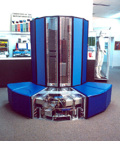
Figure 1.13. Cray-XMP (source: NSA Photo Gallery). For a color version of this figure, see www.iste.co.uk/delhaye/computing.zip
1985 saw the marketing of the Cray-2, the first computer to exceed the power of 1.7 Gflops (1.7 billion floating-point calculations per second). The machine was equipped with four processors operating at 250 MHz and had a total power of 1.9 Gflops.
In 1993, Cray produced the T3D that could be equipped with 2,048 processors and reach 300 Gflops. This was a major shift towards massively parallel architectures. It was replaced by the T3E series in 1996.
The Cray-3 was a failure and led the company to bankruptcy; it was sold to Silicon Graphics, which resold this division in 2002 to a young company, Tera Computer, which then took over the Cray name. The Cray saga was thus able to continue!
1.6.2.3. The arrival of Japanese manufacturers
Three Japanese manufacturers took their place in this rather closed circle: Hitachi, NEC, but especially Fujitsu.
Hitachi was number 1 in the 1996 TOP500 with CP-PACS/2048. The company has maintained its presence in this market while taking an increasingly smaller share. There were no Hitachi machines in the June 2019 TOP500.
In 1983, NEC introduced the SX-2, which was also a vector computer. It had a power of 1 Gflops. The SX series continued to grow while remaining faithful to the vector architecture for its processors. The latest addition, the SX-9 has a maximum power of 839 Tflops for 8,192 processors.
In 1990, Fujitsu’s VP-2600 could reach 5 Gflops with a single processor. Fujitsu built other systems, still ranked among the world’s top performers, but had a limited place in this market.
1.6.2.4. Microprocessors and massive parallelism
Early supercomputers used “homemade processors”, which were very expensive to develop and manufacture. Parallel architectures have given rise to different approaches, based on a very large number of processors, often available “off-the-shelf” and therefore inexpensive since they are produced in very large quantities for various ranges of computers.
Several companies have been created to offer massively parallel systems. One has retained the CM series (Connection Machine) of the Thinking Machine Corporation created in 1983. In its maximum configuration, the CM-5 was announced with a theoretical performance of 2 Tflops, but this efficiency was very dependent on the type of application. The complexity of programming and the reliability of these systems were fatal to these manufacturers (TMC disappeared in 1994). The major manufacturers adopted these massively parallel architectures to base their high-performance systems.
Built in 1997, ASCI Red (built by IBM for Sandia National Lab) was the first supercomputer based on “off-the-shelf” processors to take the lead in the world competition (it stayed there for four years!). In its latest version, it used 9,298 Pentium II Xeon processors with a maximum performance of 3.1 Tflops. It was stopped in 2006.
In 2004, IBM unveiled the Blue Gene/L machine, a series that would lead the competition until 2008. The latest version included more than 100,000 compute nodes for a peak performance of nearly 500 Tflops. The Roadrunner machine, built for the Los Alamos National Laboratory, followed with 20,000 hybrid PowerPC/AMD Opteron CPUs and was the first system to break the 1 Pflops barrier (peta: 1015). IBM then used, for the top end, the Power processors developed in-house.
In 2009, Cray made a strong comeback and became number one with the Jaguar XK6 machine installed at Oak Ridge National Laboratory (1.8 Pflops), which was replaced by the XK7 Titan in 2012 (more than 17 Pflops, with 18,688 AMD Opteron processors and 18,688 Nvidia GPU accelerating the high-performance computing applications).
In November 2010, the French record was held by Bull’s TERA-100, installed at CEA. With 17,296 Intel Xeon processors and a performance of 1 Pflops, this machine climbed to sixth place in the world and won first place in Europe. In 2018, TERA-1000 had a theoretical performance of 23 Pflops and was in 16th position.

Figure 1.14. The IBM Summit machine (source: Oak Ridge National Laboratory)
In November 2019, IBM was the manufacturer of the two most powerful systems in the world. The first contained 244,000 computing cores, consumed more than 10 MW of energy and could perform 148 million billion calculations in 1 second.
1.6.2.5. China, a major player since 2010
Starting in 2010, Chinese manufacturers arrived on the scene and petaflop-scale systems multiplied. In the 2019 TOP500, Lenovo PCs (remember that Lenovo acquired IBM’s PC division) accounted for 35% of the top 500 computers, but only 19% of the total installed power. Indeed, the Americans, IBM and Cray, resisted on the very high end.
In 2010, the Chinese Tianhe-1A system led the TOP500 (2.5 Pflops, 14,336 Intel Xeon CPUs and 7,168 GPUs). In 2013, the Chinese Tianhe-2 machine took the lead and stayed there for three years in a row. It was an assembly with 32,000 Intel Ivy Bridge CPUs and 48,000 Intel Xeon Phi for a total of more than 3 million cores and provided 33 Pflops. In 2016, the TaihuLight was the leading system with 41,000 Chinese ShenWei processors (260 cores per processor). It was approaching the 100 Pflops mark. In November 2019, Chinese systems occupied places 3 and 4 in the TOP500.
1.6.3. Towards exaflops
In 53 years, maximum performance has increased from 3 Mflops to 93 Pflops, a multiplying factor of 30 billion. Scientific and technological work continues, and the objective is now to reach 1 exaflop (1 billion billion operations per second). But things are not simple!
1.6.3.1. Challenges for current technologies
The first challenge is that of energy consumption. We have already said that this consumption concerns (to varying degrees) all electro-technical equipment. But with hundreds of thousands of processors, the problem becomes critical because you cannot build a nuclear power plant to run a supercomputer! The supercomputing community has admitted that the limit of consumption should be 20–30 megawatts, which is already considerable.
How to get there? Three areas are examined:
- – hardware: transistor consumption, processor architecture (in particular, associated with specialized processors such as GPUs), memory (capacity and access time), interconnection technologies, etc.;
- – software: operating systems that take consumption into account, new programming environments that make parallelism more efficient, data management, new programming environments for the scientists, etc.;
- – algorithms: reformulating scientific problems for exaflop-scale systems, facilitating mathematical optimization, etc.
1.6.3.2. Major ongoing programs
Given what is at stake, the main countries concerned are releasing considerable budgets to achieve exascale at the beginning of this new decade.
The United States, China and Japan plan to have at least one operational system by 2023. Investment in research and development is estimated at more than $1 billion per year, supported by governments and manufacturers. In August 2019, the US Department of Energy (DoE) announced the signing of a $600 million contract with Cray to install a system with a performance of more than 1 exaflop in 2022. It will be mainly intended for research on nuclear weapons.
No single country in the European Union can muster the scientific, technical and financial resources necessary to compete with Chinese or American efforts. Thus a European program is needed that involves various countries to provide the bulk of the funding and is strongly supported by the European Commission through the PRACE (Partnership for Advanced Computing in Europe) and ETP4HPC (European Technology Platform for High Performance Computing) initiatives. The aim is to have an operational system by 2023–2024, equipped with technologies that are largely European (ARM, Bull). To this end, on January 11, 2018, the European Commission announced the launch of the EuroHPC program, with initial funding of about 1 billion euros between 2018 and 2020, and a second round of funding of about 4 billion euros expected to be provided from 2021 onwards.
In all of these projects, the cost of acquiring a system would be between $300 and $400 million.
1.7. What about the future?
Then, the current technology will be at the end of its possibilities, at least to reach very high performance, and new technologies will have to be found. When will this happen? And with what constraints and consequences?
1.7.1. An energy and ecological challenge
The electricity consumption of the 14 billion computers, game consoles, set-top boxes and Internet boxes represented 616 TWh globally in 20135.
The world’s data centers account for 4% of global energy consumption, half of which is related to cooling and air-conditioning. A large data center consumes as much energy as a French city of 100,000 inhabitants.
Google is said to have more than 1 million servers in more than 10 data centers around the world. The locations are chosen according to the cooling possibilities of the machines (cold regions, proximity to vast reserves of cold water). Google has been working for a long time on the energy efficiency of its data centers and announced, in the midst of COP21, the purchase of 842 megawatts of renewable energy for its data centers, with the long-term aim of relying 100% on clean energy for its activities.
Let us not forget the consumption of cell phones and other computerized objects, produced in the billions, which use phenomenal quantities of batteries, most of which end up in landfill. Some estimate that computing (computers, networks, etc.) consumes nearly 10% of the world’s electricity consumption.
Energy consumption is not the only issue we need to consider. The materials used in computers, telephones and other objects are not neutral: various metals, elements of the rare earth family (lanthanides), whose access is considered particularly critical by international bodies, have become strategic issues. High-tech products require rare metals whose production is controlled by a limited number of countries, mainly China, Russia, the Democratic Republic of Congo, and Brazil. The scarcity and weakness of recycling can become very strong industrial and ecological constraints.
1.7.2. Revolutions in sight?
Research on totally different technologies is multiplying, both in laboratories and with processor manufacturers.
Quantum computers are the equivalent of classical computers but can perform calculations directly using the laws of quantum physics. Unlike a classical transistor-based computer that works on binary data (encoded on bits, worth 0 or 1), the quantum computer works on qubits whose quantum state can have several values. Quantum computers are so complex that they are not intended for the general public. They are useful only for very specific applications. The main practical application for a quantum computer today is cryptography.
Neuromorphic processors, inspired by the brain, are another major line of research in an attempt to create the computing power of tomorrow. They are capable of responding to the increasing computing power required by, among other things, artificial intelligence, Big Data, research in chemistry, materials science, and molecular modeling. At the end of 2017, Intel unveiled a chip called Loihi, whose architecture is inspired by the way the human brain functions, with interactions between thousands of neurons. This technology would be well suited to applications based on artificial intelligence.
Other avenues are being explored, such as the optical computer (or photonic computer), a digital computer that uses photons for information processing, while conventional computers use electrons. Other approaches exist that are essentially secret because they are studied in research laboratories.
Readers interested in this research can immerse themselves in the specialized literature.
- 1 Claude Shannon (1916–2001), an American engineer and mathematician, split his career between the Massachusetts Institute of Technology (MIT) and Bell Laboratories. In this article, he proposes a unit of information that is exactly the amount of information that a message can bring, which can only take two possible values, and with the same probability (e.g. 0 or 1).
- 2 Ada Lovelace (1815–1852) was an English scientist who anticipated the potential of the analytical machine and proposed numerous applications for it. She was the first to formalize the principle of programming, making her the first “coder” in history. It is in her honor and for the importance of her work that a programming language, designed between 1977 and 1983 for the US Department of Defense, received the name ADA in 1978.
- 3 Alan Turing (1912–1954), a British mathematician, is considered one of the fathers of computer science. In 1936, he presented an experiment that would later be called “Turing’s machine” and which would give a definition to the concept of algorithm and mechanical procedure. During World War II, he joined the British Secret Service and succeeded in breaking the secrets of German communications and the Enigma machine. After the war, he worked on one of the very first computers and then contributed to the debate on the possibility of artificial intelligence.
- 4 An engineering mathematician, John von Neumann (1903–1957) participated in the development of set theory and was a precursor of artificial intelligence and cognitive science. He also participated in American military programs. He provided decisive impetus to the development of computer science by establishing the principles that still govern computer architecture today.
- 5 Source: planetoscope.com.