(4.39)

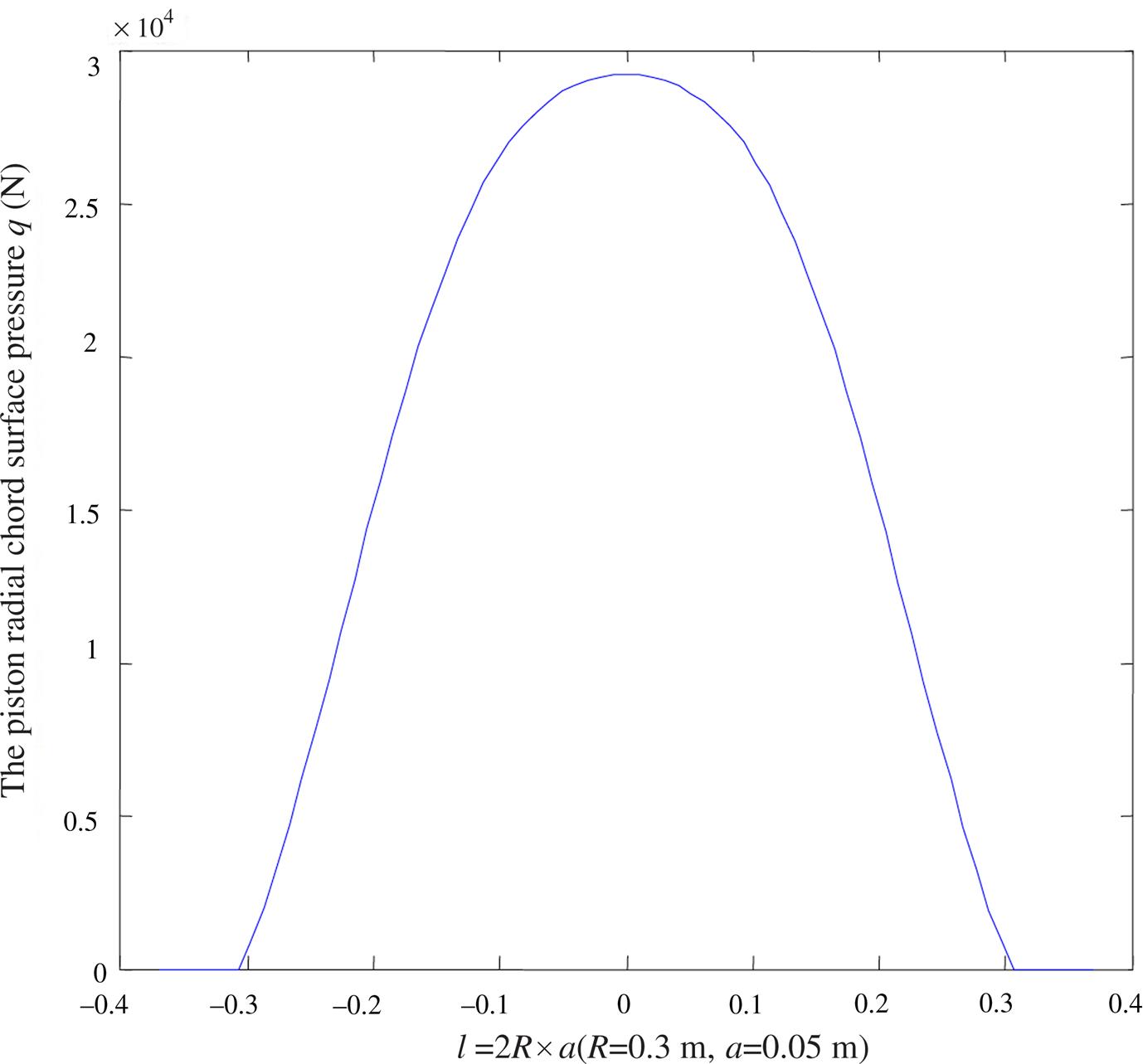
In order to verify the accuracy of the assumed radial distribution force $q_{(\theta )}$, the finite element simulation is carried out, the basic parameters are listed in Table 4.3. The piston string surface is modeled using 72 elements, and the third principle $q_{(\theta )}$ stress is chosen as the radial pressure of each point, as shown in Fig. 4.35, and then the resultant radial pressure force can be obtained to 11,465 N, Theoretical resultant force can be also obtained up to 12,203 N by using Eqs. (4.38) and (4.39). The relative error is 5%, which shows that the assumed radial distribution force $q_{(\theta )}$ is reasonable. Then, Eqs. (4.38) and (4.39) can be used to compute the final force of the piezoelectric friction damper in the following.

Assuming $F_P$ is the constraint force of the piezoelectric actuator under the electric field E, then,

$\left\{\begin{array}{l}{F}_P={\epsilon }_P{Y}_P{A}_p\\ {\epsilon }_p=\frac{\mathrm{\Delta }{L}_E}{L_p}\end{array}\right.0$ (4.40)

(4.40)

where $\mathrm{\Delta }{L}_E=d_{33}E{L}_p$ is the elongation of the actuator under the electric field E, $d_{33}$ is the axial piezoelectric strain constant, $Y_P$ is the elastic modulus of the piezoelectric ceramic, $A_p$ is the cross-sectional area of the piezoelectric ceramic actuator, $L_p$ is the axial length of the piezoelectric ceramic actuator.

$F=F_P+F_S$ (4.41)

(4.41)

where $F_S$ is the preloading force provided by spring.

Then, the positive pressure applied on the piezoelectric friction damper can be written as

$N(t)=k\times d_{33}E{Y}_p{A}_p+k\times F_s$ (4.42)

(4.42)

In order to simplify this expression, there is,

$N(t)=K{d}_{33}E+N_0$ (4.43)

(4.43)

where $K=k\times Y_p\times A_p$ is the shape coefficient of the piezoelectric friction damper, $N_0=k\times F_s$ is the pressure provided by spring. Then, the positive pressure applied on the piezoelectric friction damper can be expressed as follows

$N(t)=\left\{\begin{array}{ll}2n{N}_0\hfill & (E=0)\hfill \\ 2nK{d}_{33}E+2n{N}_0\hfill & (E>0)\hfill \end{array}\right.0$ (4.44)

(4.44)

where n is the number of spring and piezoelectric actuator.

Thus, the damping force model of the piezoelectric friction damper can be written as

$f(t)=\mu N(t)\mathrm{sgn}[\stackrel{·}{x}(t)]$ (4.45)

(4.45)

where $\mu$ is the friction coefficient between the piston and the inner surface of the outer cylinder, $\stackrel{·}{x}(t)$ is the relative velocity of the piezoelectric friction damper.

The basic parameters of the damper are listed in Table 4.4. The friction coefficient of the damper is $\mu =0.5$, preloading force of the spring is 5000 N, the number of piezoelectric actuator is 2, maximum voltage is 300 V, and maximum electric field intensity $E_0=7.5\times {10}^5\mathrm{V}/\mathrm{m}$. Based on the above analysis, the maximum damping force of the piezoelectric damper can be calculated up to 10.13 t. The theoretically computed hysteresis curves are depicted, as shown in Fig. 4.36. It can be seen that the working voltage can be adjusted real-time to get the damping force for structural vibration control.

4.4.4 Analysis and Design Methods

Assuming that a total of p piezoelectric friction dampers are installed in a structure with n degrees of freedom, the equation of motion of the controlled structure can be expressed as Eq. (2.1). The control force of the $i\mathrm{th}$ damper is in the following type:

$\{f_d(t)\}=\left\{f_{dy}\right\}\mathrm{sgn}({\stackrel{·}{x}}_d)$ (4.46)

(4.46)

where ${\stackrel{·}{x}}_d$ is the relative velocity of the piezoelectric damper, $\left\{f_{dy}\right\}$ is the variable damping force of the piezoelectric damper, and it depends on the property of the actuator and input voltage as well as the preloading force of the friction damper and the friction coefficient. The corresponding control algorithm has been introduced in the previous chapter.

A three-story reinforced concrete structure is chosen to analyze the vibration control effect of the piezoelectric friction damper, one piezoelectric friction damper is supposed to added in each floor of a three-story reinforced concrete structure, as shown in Fig. 4.37. The masses of the first, second, and third floor are $m=1.690\times {10}^4\mathrm{kg},1.581\times {10}^4\text{kg},1.412\times {10}^4\mathrm{kg}$, respectively. The stiffness of the first, second, and third floor are $k=1.512\times {10}^7\mathrm{N}/\mathrm{m}$, $2.012\times {10}^7\mathrm{N}/\mathrm{m}$, $2.012\times {10}^7\mathrm{N}/\mathrm{m}$, respectively. The Rayleigh damping ratio is adopted in this analysis procedure, the El Centro earthquake wave with a magnitude of 200 gal and the time step of 0.02 s is chosen as the excitation input. The maximum damping force provided by the damper is 158.64 kN. The analysis results are shown in Figs. 4.38 and 4.39, from which we can see that both the acceleration responses and the displacement responses are reduced significantly.

4.4.5 Tests and Engineering Applications

In recent years, piezoelectric material has been widely used in the aerospace and mechanical structure. However, piezoelectric material is mainly used as sensors in the bridge and building health monitoring in civil engineering [152–156]. Some researchers used the material to design the piezoelectric friction dampers to control the dynamic responses of the engineering structures. Qu [157] designed a piezoelectric friction damper by combining the Pall friction damper with the piezoelectric ceramic washer, of which the fastening force of the bolt can be adjusted by changing the electric-induced deformation of the washer to realize the changing of damping force, then Ou et al. [158,159] developed a T-shape PZT variable friction damper and conducted the performance test. Qu et al. [160] and Xu et al. [161] designed the friction bar with adjustable parameters by combining the piezoelectric material with the custom friction damper. Under the electric field, the deformation of the piezoelectric material is constrained, which leads to the adjustable normal pressure, thus the friction force can be adjusted real-time according to the dynamic response of the structure, then this damper was used in the practical engineering project to suppress the wind-induced vibration of Hefei Jade TV tower. Garrett et al. [162] did a lot of static and dynamic experiments on the piezoelectric friction damper, and obtained the force–displacement hysteresis curves, and the friction coefficient, equivalent damping ratio, and effective stiffness are obtained according to the experimental data, the fatigue test was also performed, the results show that the piezoelectric friction damper has a very good fatigue resistance properties. Chen et al. [163,164] also conducted the performance test of piezoelectric friction damper, and carried out the shaking table test of a quarter-scale three-story steel frame structure incorporated with piezoelectric friction dampers, results show that the piezoelectric friction damper can effectively reduce the dynamic responses of the structure. Li et al. [165,166] designed a new type piezoelectric friction damper by combining the stack type tubular piezoelectric ceramics driver and the Slotted Bolted Connection (SBC) friction damper proposed by Song [167], the prepressure was applied on the actuator through fastening bolt to restrict the deformation of the actuator, then the piezoelectric actuator can provide varied control force to realize semiactive control. Dai et al. [168] designed a piezoelectric varied friction damper by considering the commercially available multilayer piezoelectric stack actuators and the circular friction disc, this damper can provide varied damping force in each horizontal direction, and it can work together with circular seismic isolator and form smart isolation system. This damper was fabricated and performance test on this damper was also carried out. Later, the piezoelectric–Shape Memory Alloy (SMA) complex varied friction dampers [169] was designed, and experimental validation was also carried out by using a series of shaking table tests on a four-story steel isolated structure model, results showed that the damper was effective in mitigating earthquake responses on both passive-off control and the semiactive control. Wang et al. [170,171] designed a piezoelectric friction damper and conducted the performance test under different prepressure, then earthquake shaking table test was carried out to verify the control effect of the piezoelectric dampers on the dynamic responses of a transmission tower structure under El-Centrol wave excitation, results showed that the piezoelectric dampers could effectively reduce the dynamic responses of the structure.

4.5.1 Basic Principles

The working principle of semiactive variable stiffness vibration control technology is on the basis of changing the additional stiffness of the variable stiffness device in the controlled structure, so as to avoid the natural frequency of the controlled structure system being too close to or same as the excitation frequency, then to achieve the purpose of avoiding resonance of the whole system, finally to ensure that the structure is in the states of stability and security. From the point of view of energy conversion, the semiactive varied stiffness control is achieved through the deformation of the variable stiffness component so that the part of the structure vibration energy can be converted to the elastic deformation energy of the stiffness components. Then, the absorption elastic deformation energy of these stiffness elements can be released (actually, the elastic deformation energy is converted to the heat energy of the servo system), and at the same time, the part of the vibrational energy can be consumed by the damping components. Therefore, the vibration of the structure is reduced.

A typical semi-active variable stiffness control device includes three parts: additional stiffness element, mechanical device, and controller, as shown in Fig. 4.40 [172].

According to the additional stiffness component is connected or not, the variable stiffness system can produce two kinds of states: ON and OFF. The changes of the additional stiffness states (ON or OFF) can be realized by switching the controller states of the variable stiffness device according to the control algorithm.

4.5.2 Construction and Design

Based on the working principle of the semiactive variable stiffness control technology, some variable stiffness devices, as shown in Fig. 4.41, have been designed and experimentally investigated by many researchers [99,173,174]. These semiactive stiffness control devices can provide adjustable stiffness, thus the natural dynamic characteristics of the controlled structure attached to these semiactive devices can be changed.

The control force ($F_D$) of the variable stiffness device can be got from Eq. (4.47), which is calculated by analyzing the whole control system.

$\mathrm{\Delta }{K}_{\mathrm{eff}}{x}_d(t)=F_D\to F_{\mathrm{opt}}$ (4.47)

(4.47)

where $\mathrm{\Delta }{K}_{\mathrm{eff}}$ is the equivalent additional stiffness provided by the variable stiffness device, $x_d(t)$ is the displacement of the structure, and $F_{\mathrm{opt}}$ is the optimal control force of the system.

For designing the variable stiffness device, the maximum output $F_D$ is the most important index, which affects vibration control result of the structure. Take the electro-hydraulic variable stiffness device for example [175], the output force $F_D$ is associated with the piston diameter, hydro-cylinder diameter, and the oil characteristics. According to the calculated $F_{\mathrm{opt}}$, the parameters of the variable stiffness device can be optimized to get the suitable output $F_D$, which is close to the optimal control force $F_{\mathrm{opt}}$.

4.5.3 Mathematical Models

As the name suggests, the semiactive variable stiffness damper could provide additional stiffness to the controlled structure, that is, the semiactive variable stiffness damper is able to switch dynamically the working condition of the control valve, thereby dissipation or absorption of energy in the structure will take place. The parameter model of the electro-hydraulic variable stiffness damper mechanism is shown in Fig. 4.42.

These dampers can produce a large control action by dynamically changing its stiffness characteristics. When the control valve is closed, the damper serves as a stiffness element and will provide an additional stiffness to the structure. The effective stiffness $\mathrm{\Delta }{K}_{\mathrm{eff}}$ consists of $K_f$ (provided by the bulk modulus of the fluid in the hydraulic cylinder) and $K_d$ (the stiffness provided by the springs shown in Fig. 4.41B and the bracing connected with the damper). When the control valve is open, the piston is free to move and the damper will provide only certain damping ($C_e$) without stiffness. The stiffness $\mathrm{\Delta }{K}_{\mathrm{eff}}$ is the equivalent effective stiffness of the entire damper and can be calculated by

$\mathrm{\Delta }{K}_{\mathrm{eff}}=\frac{K_d{K}_f}{K_d+K_f}$ (4.48)

(4.48)

4.5.4 Analysis and Design Methods

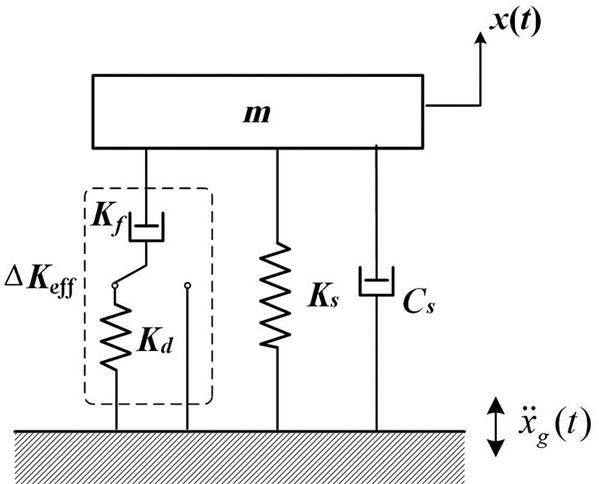
The schematic model of the semiactive variable stiffness damper used for structural vibration control of the single-freedom system is shown in Fig. 4.43, and the equation of motion of the controlled structure can be expressed as follows

$m\ddot{x}(t)+c_s\stackrel{·}{x}(t)+(k_s+\mathrm{\Delta }{k}^{*})x(t)=-m{\ddot{x}}_g(t)$ (4.49)

(4.49)

where $k_s$, $c_s$ separately are the stiffness and damping of the structure; ${\ddot{x}}_g(t)$ is the input excitation; and $\mathrm{\Delta }{k}^{*}$ is the additional stiffness provided by the semiactive variable stiffness damper.

The variable elastic force $\mathrm{\Delta }{k}^{*}x(t)$ can be moved to the right side of the motion equation as the semiactive control force, $f_d=\mathrm{\Delta }{k}^{*}x(t)$ in Eq. (4.50), which is similar to the active control force in the active variable stiffness control system.

$m\ddot{x}(t)+c_s\stackrel{·}{x}(t)+k_{s}x(t)=-m{\ddot{x}}_g(t)-f_d(t)$ (4.50)

(4.50)

According to the principle that the control forces are equal, $f_d=f_{\max }$, in which $f_{\max }$ is the optimal control force, the stiffness of the variable stiffness device can be set as

$\mathrm{\Delta }{k}^{*}=\frac{f_{\max }}{x_{\max }}$ (4.51)

(4.51)

And the additional stiffness $\mathrm{\Delta }{k}^{*}$ can be written as follows by using the switching control law

$\mathrm{\Delta }{k}^{*}=\left\{\begin{array}{ll}\mathrm{\Delta }{k}_{\mathrm{eff}}\hfill & \mathrm{OFF}\hfill \\ 0\hfill & \mathrm{ON}\hfill \end{array}\right.0$ (4.52)

(4.52)

where $\mathrm{\Delta }{k}^{*}=\mathrm{\Delta }{k}_{\mathrm{eff}}$, if the switch is closed; and $\mathrm{\Delta }{k}^{*}=0$, if the switch is open. The equivalent effective stiffness $\mathrm{\Delta }{k}_{\mathrm{eff}}$ can be calculated from Eq. (4.48).

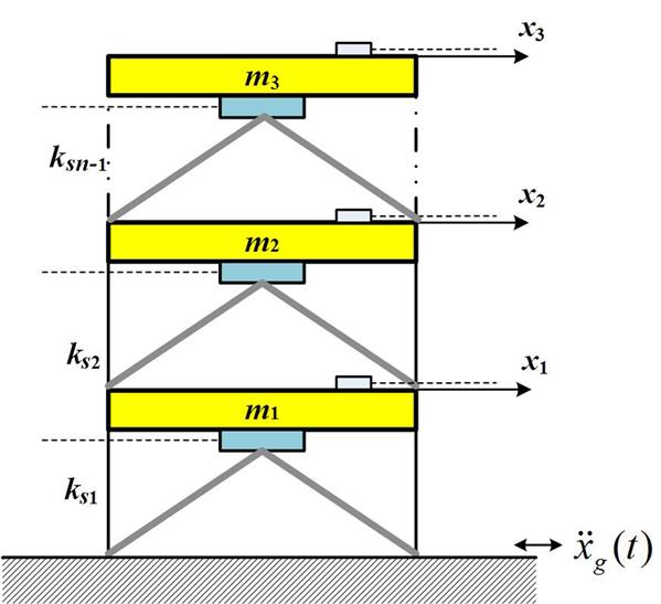
There are p semiactive variable stiffness devices installed in an n stories structure, as shown in Fig. 4.44. The equations of motion of the linear, n-story building structure equipped with semiactive variable stiffness system can be expressed as follows

$\left\{\begin{array}{l}\left[M\right]\{\ddot{x}(t)\}+\left[C\right]\{\stackrel{·}{x}(t)\}+\left[K\right]\{x(t)\}=\{P(t)\}+\left[B\right]\{f_d(t)\}\\ x(t_0)=x_0\stackrel{·}{x}(t_0)={\stackrel{·}{x}}_0\end{array}\right.0$ (4.53)

(4.53)

where the meaning of each item is the same as Eq. (2.1).

Eq. (4.53) can be represented in the state-space form as

$\left\{\begin{array}{l}\{\stackrel{·}{Z}(t)\}=\left[A\right]\{Z(t)\}+\left[D_0\right]\{P(t)\}+\left[B_0\right]\{f_d(t)\}\\ \left\{Y\right\}=\left[E_0\right]\{Z(t)\}\end{array}\right.0$ (4.54)

(4.54)

where the meaning of each part is the same as Eq. (2.5).

The semiactive control force of these semiactive variable stiffness dampers u_i (i=1, 2,…, p) can be calculated as

$u_i(t)=\mathrm{\Delta }{k}_i{g}_i(t)x_i(t)$ (4.55)

(4.55)

In Eq. (4.55), the $g_i(t)$ expressed for switching control law as

$g_i(t)=\left\{\begin{array}{ll}1\hfill & ({\stackrel{·}{x}}_i{x}_i>0)\hfill \\ 0\hfill & ({\stackrel{·}{x}}_i{x}_i\le 0)\hfill \end{array}\right.0$ (4.56)

(4.56)

Therefore, the variable stiffness $\mathrm{\Delta }{k}_i$ of the dampers can be calculated according to the equivalent principle of which the control force is equal, as seen Eq. (4.51).

4.5.5 Tests and Engineering Applications

Generally, a semiactive stiffness damper consists of a fluid-filled cylinder, a piston, and a motor-controlled valve. Based on the feedback information of structural responses, the motor regulates the valve open or close to dissipate or absorb vibration energy of the structures. A significant amount of researches and developments have been conducted on semiactive variable stiffness devices. Li and Liu [176,177] conducted a shaking table test of semiactive structural control using variable stiffness, which is set in the 1:4 model of a five-story frame, the test results showed that this type of control system was capable of efficiently reducing the structural vibration response. Kobori and Nasu [178,179] also conducted shaking table test of the structure incorporated with the variable stiffness system, results showed that the device used was efficient. Kumar et al. [180] used the semiactive control variable stiffness damper (SAVSD) to control the vibration of piping system used in industry, fossil and fissile fuel power plant, and the SAVSD changed its stiffness depending upon the piping response and accordingly added the forces in the piping system. Nasu et al. [181] experimentally studied a high-rise building with variable stiffness system. The model of the building is a 25-floor steel frame structure, and test results showed that the variable stiffness system needed only a little external energy and can reduce the responses of the structure efficiently. The resetting semiactive stiffness dampers designed for controlling a 2D, three-story, three-bay frame under random excitations were experimentally studied by Jabbari and Bobrow [182]. A semiactive control system with the switching semiactive stiffness dampers used for controlling a 2D, 20-story frame under two different earthquake waves were studied by Kurino et al. [183]. Similarly, some other tests on the semiactive control systems with different semiactive stiffness dampers and different control strategies have been conducted in succession [184–186].

The varied stiffness system [187] was designed to prevent resonance with the seismic motion, by means of controlling the stiffness of the building through a control computer (nonstationary, nonresonant), according to the ever-changing properties of the seismic motion. The building was thus protected from the destructive energy of the earthquake. The control computer instructed the varied stiffness damper how to alter the stiffness of each story to reduce the response of the building by preventing its resonance with the seismic motion, through the selection of different stiffness types. Application of the semiactive variable stiffness damper has been investigated for a cable-stayed bridge, shown in Fig. 4.45A [188]. In the research, a resetting semiactive stiffness damper, shown in Fig. 4.45B, was used to control the peak dynamic response of the cable-stayed bridge subject to earthquakes. It is shown that the designed damper is quite effective on reducing peak response quantities of the bridge. The tests and application of previous studies indicate that the semiactive variable stiffness device is effective in reducing structural responses.

4.6.1 Basic Principles

The varied damping damper system is firstly proposed by Hrovat [98], the damping is adjusted in real-time by using the additional damping device. The classical varied damping damper is shown in Fig. 4.46. It consists of a hydraulic cylinder, a piston, and an electro-hydraulic servo valve. Only very small energy is needed to adjust the opening size of the servo valve, and the damping force can be achieved to 100–200 t.

The damping force provided by the varied damping damper depends on the opening size of the servo valve. As shown in Fig. 4.46, when the valve is completely open, the damper can provide minimum damping force, named the passive-off state. On the contrary, the maximum damping force is provided when the servo valve is completely closed, which is called the passive-on state. The range of damping force provided by the damper is between the passive-off and passive-on state, and can be adjusted according to the dynamic response of the structure.

4.6.2 Construction and Design

Based on the working principle of the semiactive variable damping control technology, some variable damping devices have been designed and experimentally investigated by many researchers [189–192]. These semiactive variable damping dampers are utilized to adjust the damping so that the dynamic responses of the structure can be reduced to meet the demand.

Symans and Constantinou [193] designed a variable damping damper based on the passive viscous fluid damper, as shown in Fig. 4.47. This device consists of oil cylinder with oil inlet and outlet, piston with small holes, bypass pipeline with the servo control system and the accumulator. The servo control system is a coil using closed-loop control. When the small hole of the bypass pipe is closed, the fluid will flow directly from one oil chamber to the other oil chamber through the small hole in the piston, and will not flow from the bypass pipe. At this time, this device is equivalent to the traditional passive viscous fluid damper and can provide the largest damping coefficient $c_{d\max }$. When the small hole in the bypass pipe is opened completely, then the fluid will flow from one chamber to another chamber through both holes in the piston and the bypass pipe. The device is also equivalent to the traditional passive viscous fluid damper, but it provides the smallest damping coefficient $c_{d\min }$. By adjusting the opening size of the hole of the bypass pipe, the damping coefficient of the device varies from the smallest with closed holes to the largest with completely open holes in the bypass pipeline.

4.6.3 Mathematical Model

The variable damping damper is actually like a hydraulic system, thus the mathematical model can be established using the fluid mechanics theory according to the oil circuit structure. The classical variable damping device will be employed to introduce the modeling method [194], and the computing model is shown in Fig. 4.48.

Assuming the force applied on the piston is $u_d$ and the relative velocity is $\stackrel{·}{x}$, the effective area of the piston is $A_p$, the pressure of the two cavities are $p_1$, $p_2$, and the corresponding volumes are $V_1$, $V_2$. The damping coefficient is $c_v$ (adjustable, with respect to voltage).

According to the force balance of the piston rod, the control force of the device can be written as follows:

$F=A_p(p_2-p_1)$ (4.57)

(4.57)

Assuming the fluid in the servo valve is incompressible, the pressure is linear to the flow, then,

$Q_1=Q_2,p_2-p_1=c_{v}Q$ (4.58)

(4.58)

Assuming the fluid in the hydraulic cylinder is compressible, the volume elastic modulus is $\beta$, then the volume change due to the pressure change is

${\stackrel{·}{p}}_1{V}_1=-\beta {\stackrel{·}{V}}_1,{\stackrel{·}{p}}_2{V}_2=-\beta {\stackrel{·}{V}}_2$ (4.59)

(4.59)

where the minus sign represents the decrease of fluid volume.

The flow change rates are as follows:

${\stackrel{·}{V}}_1=-Q_1+A_p\stackrel{·}{x},{\stackrel{·}{V}}_2=Q_2-A_p\stackrel{·}{x}$ (4.60)

(4.60)

Based on the above equations, the pressure change rate in the two cavities due to the motion of the piston rod is [194]

${\stackrel{·}{p}}_2=-\frac{\beta }{V_2}\frac{F}{A_p{c}_v}+\frac{\beta }{V_2}{A}_p\stackrel{·}{x}$ (4.61)

(4.61)

$-{\stackrel{·}{p}}_1=-\frac{\beta }{V_1}\frac{F}{A_p{c}_v}+\frac{\beta }{V_1}{A}_p\stackrel{·}{x}$ (4.62)

(4.62)

Combining the above two equations, the rate of the pressure drop is

${\stackrel{·}{p}}_2-{\stackrel{·}{p}}_1=-\frac{\beta }{A_p{c}_v}\left(\frac{1}{V_1}+\frac{1}{V_2}\right)F+\beta A_p\left(\frac{1}{V_1}+\frac{1}{V_2}\right)\stackrel{·}{x}$ (4.63)

(4.63)

According to Eq. (4.57), the controllable control force of the varied damping damper can be written as follows:

$\stackrel{·}{F}=\frac{k_d}{c_d}F+k_d\stackrel{·}{x}$ (4.64)

(4.64)

where $k_d=4\beta A_p^2/V_T$ is the stiffness of the hydraulic system, $V_T=4{((1/V_1)+(1/V_2))}^{-1}$, $c_d=c_v{A}_p^2$ is the damping coefficient of the hydraulic system. Eq. (4.64) is the final computing equation of the damping force of the varied damping device.

4.6.4 Analysis and Design Methods

The schematic model of the semiactive variable damping damper used for structural vibration control of the single-freedom is shown in Fig. 4.49. According to the damping force type provided by the device, the motion equations of the controlled structure can be expressed as follows

$\mathrm{uncontrolled}m\ddot{x}+c\stackrel{·}{x}+kx=f$ (4.65)

(4.65)

$\text{Passive}-\text{on}m\ddot{x}+(c+c_{d\max })\stackrel{·}{x}+kx=f$ (4.66)

(4.66)

$\text{Passive}-\text{off}m\ddot{x}+(c+c_{d\min })\stackrel{·}{x}+kx=f$ (4.67)

(4.67)

$\text{Semi}-\text{active}m\ddot{x}+c\stackrel{·}{x}+kx+c_d(v,t)\stackrel{·}{x}=f$ (4.68)

(4.68)

where $f$ is the disturbance, $c_d(v,t)$ is the damping coefficient with respect to voltage and time provided by the varied damping damper. A three-story frame structure is adopted to analyze the control effect of varied damping dampers. The mass and story stiffness are $m_i=4\times {10}^5\mathrm{kg}$, $k_i=2\times {10}^8\mathrm{N}/\mathrm{m}$, respectively. The Rayleigh damping ratio is adopted and the first two damping ratios are both 0.05. EI Centro wave is employed with a peak value of 200 gal. Three varied damping dampers are arranged at each story, the maximum damping coefficient of the three semiactive varied damping dampers are $c_{1d\max }=7.7012\times {10}^6\mathrm{N}\cdot \mathrm{s}/\mathrm{m}$, $c_{2d\max }=7.7232\times {10}^6\mathrm{N}\cdot \mathrm{s}/\mathrm{m}$, $c_{3d\max }=5.42\times {10}^6\mathrm{N}\cdot \mathrm{s}/\mathrm{m}$, the minimum damping coefficients of the three dampers are $c_{1d\min }=9.6265\times {10}^5\mathrm{N}\cdot \mathrm{s}/\mathrm{m}$, $c_{2d\min }=9.6539\times {10}^5\mathrm{N}\cdot \mathrm{s}/\mathrm{m}$, $c_{3d\min }=6.7716\times {10}^5\mathrm{N}\cdot \mathrm{s}/\mathrm{m}$. The additional damping ratio due to the damper (passive-off state) is 2.34%, the maximum responses under different control strategy are listed in Table 4.5.

In order to realize semiactive control, the optimal Bang-Bang control strategy, which can be expressed as:

$c_d(t)=\left\{\begin{array}{ll}{c}_{d\max }\hfill & u\stackrel{·}{x}<0\hfill \\ c_{d\min }\hfill & u\stackrel{·}{x}\ge 0\hfill \end{array}\right.0$ (4.69)

(4.69)

According to Table 4.5, results show that both the displacement and acceleration responses of the structure are reduced by using passive-off control and semiactive control. Comparatively speaking, the passive-off control method can only reduce the dynamic responses in a small extent, while the acceleration and displacement responses of the structure using semiactive control can be reduced by 30–40%, which shows that semiactive control can achieve excellent control effect. In addition, the control effect of passive-off algorithm is dominated by the design of the minimum damping coefficient $c_{id\min }(i=1,2,3)$. Apparently, the control effect will be more significant with increasing $c_{id\min }$.

4.6.5 Tests and Engineering Applications

A significant amount of research and developments have been conducted on semiactive variable damping devices. Kawashima [192], Symans and Constantinou [193], and Niwa [190] conducted a series of mechanical tests on the varied damping dampers under different excitation frequencies and amplitudes, and obtained the force–displacement hysteresis curves. Symans [193] conducted a shaking table test on a three-story steel frame structure incorporated with variable damping dampers. The geometric similarity ratio between the model and the prototype is 1:4, the whole mass of the structure is 2868 kg with 956 kg for each layer. The variable damping device is installed at the bottom of the structure, and the dynamic responses can be measured using the acceleration sensors and displacement sensors. Research results show that the variable damping devices can significantly reduce the dynamic responses of the structures. Niwa and Kobori [190] used the variable damping damper to control a steel office building located at Shizuoka city. Eight dampers were installed at the gable of one to four layers, and results show that the designed damper can significantly increase the damping of the structure and is quite effective in reducing peak response quantities of the steel structure. As we know, the long-time vehicle loading on the bridge will lead to the fatigue effect, thus the variable damping damper is especially suitable for vibration control of the bridge structure. Kawashima [192], Shinozuka [195], Patten [196], and Gavin [194,197] conducted a lot of researches on the vibration control of bridges using variable damping device. Patten firstly took the variable damping device into actual engineering project to reduce the vibration of a I-35 Bridge in America, and results show that the semiactive variable damper has an excellent control effect, and the minimum service life can be extended by 35.8 years. Li et al. [198] developed a kind of fluid viscous semiactive damper and experimentally studied the performance of the controller of the semiactive damper, then a 1:4 scale five-story steel structure with and without the semiactive damper was tested using a shaking table under EL-Centro and Tianjin earthquake ground excitations, in which the control laws of Hrovat and ON/OFF algorithms were used. The results indicated that semiactive damper reduced earthquake responses significantly. Yang et al. [199] studied the effectiveness of using a semiactive variable damper to control seismically excited structures, and results show that the performance of variable dampers in reducing the seismic response of structures depends on the ratio of the disturbance frequencies to the natural frequencies of structures, rather than the natural frequencies of structures only.

The above tests and application of previous studies indicated that the semiactive variable damping damper was effective in reducing structural responses.

4.7.1 Basic Principles

It can be seen from the composition of MRE that the MRE is a kind of composite material, which is made of magnetized particles dispersed in a solid polymer medium such as rubber. Under the external magnetic field, the matrix is cured, then the magnetic particles are locked into a place and the chains are firmly established in the matrix. The elastic modulus of an MRE increases monotonically with the strength of the magnetic field. Upon removal of the magnetic field, the MRE immediately reverts to its initial status. The changed modulus of MRE caused by a magnetic field is called magnetic-induced modulus, which affects the adjustability of the MRE, so it is an important index of MRE properties.

In order to explain the causes of the magnetic effect of MREs and provide the theoretical basis for improving the performance of MRE. The microphysical model is proposed by some researchers from different angles. This kind of microphysical model, such as magnetic dipole model, coupling field model, single chain model and so on, can simulate the magnetic-induced modulus of MREs.

Magnetic dipole model [206]:

$\mathrm{\Delta }G=\frac{(4{\gamma }^4-27{\gamma }^2+4)\mathrm{\Phi }{J}_p^2}{8{\mu }_1{\mu }_0{r_0}^3{({\gamma }^2+1)}^{9/2}}$ (4.70)

(4.70)

Coupling field model [207]:

$\mathrm{\Delta }G=\frac{9}{8}\frac{\mathrm{\Phi }C|m_i{|}^2(4-{\gamma }^2)}{r_0^3{\pi }^2{d}^3{\mu }_1{\mu }_0{(1+{\gamma }^2)}^{7/2}}$ (4.71)

(4.71)

Single chain model [208]:

$\mathrm{\Delta }G=\frac{9\mathrm{\Phi }|m_i{|}^2\zeta }{4{\pi }^2{d}^3{r}_0^3{\mu }_1{\mu }_0}$ (4.72)

(4.72)

where $\mathrm{\Delta }G$ is the magnetic-induced modulus of the MRE, $\mathrm{\Phi }$ is the volume ratio of magnetic particles, $r_0$ is the distance between two magnetic particles, $d$ is the magnetic particle diameter, $\gamma$ is the shear strain, $\left|m_i\right|$ is the magnetic dipole moment, and $J_p$ is the intensity of the polarization of magnetic particles.

It can be seen from the microphysical model that the magnetic modulus is affected by many factors, such as the volume ratio of magnetic particles $\mathrm{\Phi }$, the distance between two magnetic particles $r_0$, the magnetic particles diameter $d$, the shear strain $\gamma$, the external magnetic field H, and so on. The $\mathrm{\Phi }$, $r_0$, and $d$ decide the performance of MRE when the MRE is prepared, whose magnetic modulus mainly affected by the shear strain $\gamma$ and the external magnetic field H.

According to different stress states, the operation modes of MRE can be divided into shear mode and tension-compression mode. The schematic diagram of MRE’s operation mode is shown in Fig. 4.50.

The tension-compression mode, as shown in Fig. 4.50A, in which the pole plate carry through relative movements in the direction parallel to the field, and the MRE is in the alternation state of tensile and compression. Due to the relative movement of the magnetic pole plates, the magnetic field strength, between the two pole plates, changes continuously, so as to achieve the purpose of changing the properties of MRE. However, due to the coupling between the magnetic nonlinear of magnetic field and magnetic particles, the MRE device system with tension-compression mode is very complicated and it is difficult to design, therefore, there is few devices designed in the tension-compression mode.

The MRE in shear mode placed in the two pole plates is shown in Fig. 4.50B: one pole plate is fixed and another moves in the direction perpendicular to magnetic field. So, the mechanical properties can be changed by controlling the external magnetic field. Due to that the distance between the two pole plates is very small and constant, then, it is easy to form a relatively uniform magnetic field, so it is relatively simple to design the MRE device system with the shear mode. At present, most of the MRE devices adopt the shear operation mode.

4.7.2 Construction and Design

Based on the shear operation mode, different kinds of MRE devices are designed and studied, such as vibration absorbers [209], vibration damping devices [210–212], and so on, shown in Fig. 4.51.

For these MRE devices designed in the form of shear mode, the shear stiffness K which is an important parameter in structural vibration control and can be expressed as follows

$K=K_0+\mathrm{\Delta }K=\frac{G_{0}A}{h}+\frac{\mathrm{\Delta }GA}{h}$ (4.73)

(4.73)

where $G_0$ is the initial shear modulus of MRE and $\mathrm{\Delta }G$ is the magnetic-induced shear modulus. In Eq. (4.73), $\mathrm{\Delta }K$ is the increment of stiffness caused by the magnetic-induced shear modulus $\mathrm{\Delta }G$, which is an important index for MRE device design and affects the adjustability of MRE devices.

It can be seen from Fig. 4.51 that all kinds of MRE devices consist of two parts: MRE material and magnetic circuit structure.

4.7.3 Mathematical Models

So far, many researchers have theoretically and experimentally studied MRE devices under external magnetic field. In order to realize the calculation of structures incorporated with MRE devices, a mathematical model should be deduced to describe the performance of MREs under a magnetic field. Till now, some models were proposed in analyzing the field-dependent modulus of MREs based on simple chain mechanisms and particle dipole interactions, as mentioned in Section 4.7.1. These microphysical models [206–208] were proposed to calculate the magnetic-induced modulus of MRE. These models are deduced from the microaspect, and can be used to calculate the magnetic-induced shear modulus. However, the final purpose of proposing these models is to explain the macroscopic mechanical behavior of MRE and can be used to simulate force–displacement of MRE devices. Thus, the macromodel of MRE device should be proposed.

From these experimental results, we can see that the MRE material exhibits a feature that its modulus and damping capability are both magnetic field dependent, and the behavior of MRE without an external magnetic field processes the viscoelastic property. Generally speaking, the mechanical behaviors of MRE can be described as magnetic-induced viscoelastic property. Based on the viscoelastic theory, some parametric models were proposed to describe the magnetic-induced viscoelastic properties of MRE. A constitutive model was derived based on the viscoelasticity theory, in which four variables are adopted in the constitutive function to capture the viscoelastic characteristics of the matrix and the magnetic-induced effect [215]. Another four-parameter linear viscoelastic model was proposed, which could predict the dynamic mechanical property of MRE performance under various working conditions [216]. In addition, a fractional derivative magnetic viscoelastic parameter model was proposed to describe the magnetic viscoelastic mechanical behavior of MR elastomers under external magnetic field [217]. These macroparameter models are shown in Fig. 4.52.

It can be seen from Fig. 4.52 that several simple mechanical components, such as the spring element and so on, are combined together in the form of series or parallel. The physical interpretations of these mechanical elements in these models separately are the shear modulus of the matrix (spring element), the damping coefficient of MRE (Newton pot element), and the magnetic-induced shear modulus of MRE (nonlinear spring element). Then, the constitutive equations of these models were built, and take the fractional derivative magnetic viscoelastic parameter model for example. Supposing the input strain is ε, while the output stress is σ, the constitutive equation can be expressed as follows

$\sigma (t)=G_0\epsilon (t)+G_0{\tau }^{\alpha }{D}^{\alpha }[\epsilon (t)]+G_m(H)\epsilon (t)+\mu G_m(H)\tau \stackrel{·}{\epsilon }(t)$ (4.74)

(4.74)

where α is the fractional order. In order to get the complex modulus G*, the Fourier transformation is undertaken for Eq. (4.74), then

$G^{*}=\frac{\sigma (\omega )}{\epsilon (\omega )}=G_0+G_0{\tau }^{\alpha }{(i\omega )}^{\alpha }+G_m(H)+i\mu G_m(H)\tau \omega =G_1(\omega )+i{G}_2(\omega )$ (4.75)

(4.75)

where G₁ and G₂ are real and imaginary parts of the complex modulus, respectively. The $i^{\alpha }=\cos (\alpha \pi /2)+i\sin (\alpha \pi /2)$ is undertaken for Eq. (4.75), then the storage modulus G₁ and loss modulus G₂ can be obtained

$G_1=G_m(H)+G_0\left(1+{\tau }^{\alpha }{\omega }^{\alpha }\cos \frac{\alpha \pi }{2}\right)$ (4.76)

(4.76)

$G_2=\mu G_m(H)\omega \tau +G_0{\tau }^{\alpha }{\omega }^{\alpha }\sin \frac{\alpha \pi }{2}$ (4.77)

(4.77)

and the loss factor can be calculated

$\eta =\frac{G_2}{G_1}=\frac{\mu G_m(H)\omega +G_0\tau {\omega }^{\alpha }\sin (\alpha \pi /2)}{G_m(H)+G_0\left(1+\tau {\omega }^{\alpha }\cos (\alpha \pi /2)\right)}$ (4.78)

(4.78)

where ω is the excitation frequency.

The parameters in the equations can be identified by using the experimental data, then the equivalent stiffness used in the structural vibration control analysis can be calculated by Eq. (4.73).

4.7.4 Analysis and Design Methods

4.7.4.1 MRE vibration absorber

The dynamic vibration absorber is a tuned spring-mass system, which reduces or eliminates the vibration of a harmonically excited system. The working principle of the dynamic vibration absorber, as shown in Fig. 4.53A, is added to the mass spring system on the vibration objects. In order to let the amplitude of the primary system be zero, the design working frequency of the vibration absorber should be close to the excitation frequency. The design working frequency is

$f_a=\frac{1}{2\pi }\sqrt{\frac{K_2}{m_2}}\to f_e$ (4.79)

(4.79)

From Eq. (4.79), we can see that the working frequency of the ordinary vibration absorbers is one fold or narrow brand. The working frequency of MRE vibration absorber can be changed in real time because the stiffness is controllable under external magnetic field. That is to say, the working frequency can be designed to trace the excitation frequency by changing the shear modulus of MRE. Therefore, combined with Eq. (4.73), the working frequencies can be designed by optimizing these parameters of A, h, and m.

4.7.4.2 MRE damping device

As a kind of semiactive vibration control device, the working principle of MRE is the same as that of MR damper, which can provide a “control force” F to the whole system. Fig. 4.53B is the working principle of the MRE vibration damping device, in which F can be expressed as follows

$F_{\mathrm{MRE}}=\mathrm{\Delta }K\cdot s\tau$ (4.80)

(4.80)

where $\mathrm{\Delta }K=d{I}^2+eI+f$, d, e, f separately are the constants fitted by the experimental data, and $s\tau$ is the shear deformation.

Based on the design experience of MR damper, the elastic force F (control force), similar to the damping force of MR damper, is the most important index for designing MRE damping devices. From Eq. (4.73), we can see that $\mathrm{\Delta }K=\mathrm{\Delta }GA/h$ is the stiffness increment of MRE device produced by the magnetic-induced shear modulus.

From the microphysical model, we can see that the magnetic-induced shear modulus $\mathrm{\Delta }G$ is mainly affected by the external magnetic field H when the MRE material is prepared. So, a reasonable magnetic circuit structure is needed to provide a uniform and enough magnetic fields for MRE working area, as seen in Fig. 4.54.

4.7.5 Tests and Engineering Applications

Since 1995 MREs were found, a series of the performance experiments of MREs were conducted and some of the MRE devices, such as, controllable stiffness of car bushing and adjustable vibration absorber were designed, which were used and applied for patents [218–220]. Shiga et al. [221] prepared two MRE samples using the silicon rubber as the matrix, then the mechanical properties of the MRE were studied with parallel plate shear model test. Jolly et al. [222] examined the mechanical response of elastomer composites subjected to magnetic fields, and these elastomer composites consist of carbonyl iron particles embedded within a molded elastomer matrix. The composite is subjected to a strong magnetic field during curing, which causes the iron particles to form columnar structures that are parallel to the applied field. Lokander and Stenberg [223] studied the ways to increase the MR effect, results showed that the absolute MR effect of isotropic MR rubber materials with large irregular iron particles was independent of the matrix material, and the relative MR effect could be increased by the addition of plasticizers. Of course, the MR effect can be increased by increasing the magnetic field, although the material saturation will emerge at large fields. Mysore [224] prepared two types of MRE with different concentrations, and circular and rectangular shapes having thicknesses from 6.35 mm to a maximum of 25.4 mm, and these samples were tested under quasi-static compression and quasi-static double lap shear. The results showed that the measured off-state shear modulus had large variations with increase in the thickness of the sample, and the measured shear modulus from the double lap shear test results, as well as the Young's modulus from the compression tests at zero-field, followed a logarithmic trend. An adaptive variable stiffness MRE absorber was developed by Dong et al. [225], and the working characteristics of this developed MRE absorber were also tested in a two-degree-of-freedom dynamic system. In addition, an active-damping-compensated MRE adaptive tuned vibration absorber was proposed by Gong et al. [226] and the dynamic properties and vibration attenuation performances were also experimentally investigated. Li et al. [210] designed a continuously variable stiffness MRE isolator used in vehicle seat suspension and the vibration control effect of the MRE isolator was evaluated. An isolation bearing with MRE used for structural vibration control in civil engineering was designed by Tu et al. [227].

Recently, for the deeper research on magnetic-characteristics and a wider range of applications of MRE, experimental researches on mechanical performance of MREs, especially on shear performance, have been studied, the results of which provide theoretical basis for the MRE devices with the shear working mode. The shear performances of MRE, that is, the dynamic viscoelastic properties under different magnetic fields, displacement amplitudes, and frequencies, were tested by the equipment, similarly as shown in Fig. 4.55. For example, the MRE fabricated with bromobutyl rubber and natural rubber was designed by Xu et al. [228] and the performances of the kind of MRE devices was tested, in which the test sample was manufactured in a style of a sandwich, as shown in Fig. 4.56.

These MRE samples were tested with respect to harmonic loadings in accordance with various displacement amplitudes (1, 2, and 4 mm) and frequencies (1, 2, 5, and 10 Hz). Originally, the experimental force displacement traces were recorded and only one cycle was taken for the calculations to ensure that the values represented only the steady state, and the test process is shown in Fig. 4.57. Figs. 4.58–4.60 show the force–displacement hysteresis curves of the two MREs under different currents, displacement amplitudes, and excitation frequencies.

Fig. 4.58 shows the force–displacement relationships of the two kinds of MRE samples (take NR70 and BIIR70 for example) at the constant displacement amplitude of 2 mm, frequency of 10 Hz but at various magnetic fields from 0 to 300 mT. From this figure, we can see that the hysteresis loops of the two kinds of MRE can shape ellipses, and the slope of the major axis of the elliptical loops varies with the magnetic field. The experimental force F increases with the increment of magnetic field strength values while the displacement amplitude is constant. This means that because of the changes in the material, a greater force is required to maintain the same level of displacement, that is to say, the stiffness of MREs varies with the magnetic fields. The areas of the elliptical loops increase slightly with the increment of the magnetic fields, which demonstrates that the damping capacity of the MRE samples is a function of the applied magnetic fields.

Fig. 4.59 shows the force–displacement curves of the MRE samples, NR60 and BIIR60, at the constant displacement amplitude of 2 mm, magnetic fields of 200 mT but at various frequencies from 1 to 10 Hz. It can be seen from these figures that the changes in slope of the main axis of hysteresis loops are not significant, whereas the loops area increases markedly, which demonstrates that the damping capacity of the MRE specimens is greatly influenced by the excitation frequencies.

Fig. 4.60 shows the force–displacement curves of NR70 and BIIR70 at the constant frequency of 2 Hz, the magnetic field of 200 mT but at various displacement amplitudes. It can be seen from Fig. 4.60 that the slopes of the main axis of these elliptical loops obviously change with the increment of the displacement amplitudes, which means that the stiffness of MRE specimens decreases when the displacement amplitudes increase from 1 to 4 mm.

Due to the controllable performance of MRE devices, they have been used in the automobile suspension system to reduce the deformation of the suspension system and increase the comfortableness [219]. However, the MRE devices used in the practical civil engineering projects have not been reported as far as the author concerned, and literatures are only limited in theoretical and experimental analysis. Along with the deepening of researches, the performance of MRE will be improved and may be used in the practical engineering project in the future.