
Example and Program Analysis
Abstract
The control algorithm and theoretical dynamic analysis method of the intelligent controlled structure have been presented in detail in the previous chapters; this chapter will focus on the specific numerical examples. The building structure with magnetorheological (MR) dampers, the bridge with MR dampers, and the platform with MR elastomer devices are chosen to evaluate the control effects of the semiactive intelligent control devices. The building structure with active tendon system is taken as an example to verify the control effect of active control.
Keywords
Numerical example; intelligent controlled structure; semi-active control; active control
How to solve the real problems of intelligent vibration control in civil engineering structures is a comprehensive application of knowledge described in the previous chapters. Some examples about intelligent vibration control in different civil engineering structures with different kinds of intelligent control devices will be presented to narrate semiactive control and active control.
8.1 Dynamic Analysis on Frame Structure With MR Dampers
8.1.1 Structural and Damper Parameters
A 10-story reinforced concrete frame structure in the 8 degree area is chosen to evaluate the control effect of the magnetorheological (MR) damper. The height of the bottom layer is 5 m, the height of the other layers is all 3.2 m, and the spans from left to right are 8.4 m, 5.4 m, and 7.2 m, respectively. The cross section of the column for the first to the sixth story is ![]() mm, and
mm, and ![]() mm for 7–10 layers. The sizes of the beams are 250×550 mm, 250×600 mm, and 250×650 mm, respectively, and the damping ratio is chosen as 0.05. The structure diagram and the reinforcement figures are shown in Fig. 8.1.
mm for 7–10 layers. The sizes of the beams are 250×550 mm, 250×600 mm, and 250×650 mm, respectively, and the damping ratio is chosen as 0.05. The structure diagram and the reinforcement figures are shown in Fig. 8.1.

The elastic time-history analysis is performed using the beam-column model. The MR dampers are installed in the middle span in the bottom six floors, as shown in Fig. 8.2. El Centro wave and Taft wave with a modified peak value of 140 gal are chosen as earthquake excitations. The maximum force of the MR damper is 200 KN, and the viscous damping coefficient is cd=60 KN s/m. The consistent mass matrix and Rayleigh damping matrix are employed. The dynamic responses of the structure under the condition of passive-off control, semiactive control, and uncontrolled are calculated by MATLAB programming, among which the passive-off control means the MR damper control with no current input and only the viscous damping force is provided.

8.1.2 Semiactive Control Strategy
MR damper, as a semiactive control device, cannot provide the optimal control force at any instant, thus the following control strategy is adopted to realize semiactive control, as shown in Eq. (8.1). It can be seen that the damper will provide the maximum force when the optimal control force is larger than the maximum force and its direction is different from the velocity of the damper; similarly, the damper will provide the minimum force when the optimal control force is smaller than the minimum force and its direction is the same as the velocity of the damper; for other conditions, the damper will provide the optimal control force, which is calculated using the linear quadratic regulator (LQR) optimal control algorithm discussed in Chapter 2, Intelligent Control Strategies.
(8.1)
 (8.1)
(8.1)
where ![]() ,
, ![]() are the minimum and maximum damping force provided by the
are the minimum and maximum damping force provided by the ![]() MR damper,
MR damper, ![]() ,
, ![]() are the displacement and velocity of the
are the displacement and velocity of the ![]() MR damper,
MR damper, ![]() is the optimal control force calculated by LQR optimal control algorithm,
is the optimal control force calculated by LQR optimal control algorithm, ![]() is the damping force provided by the ith MR damper. Fig. 8.3 shows the semiactive control strategy.
is the damping force provided by the ith MR damper. Fig. 8.3 shows the semiactive control strategy.

8.1.3 Results and Analysis
Dynamic responses of the structures with and without MR dampers can be got through elastic time-history analysis. Fig. 8.4 shows the displacement and acceleration time-history responses of the top node (node 40). It can be seen that the peak values of the displacement responses are reduced by 23.4% and 44.1%, respectively, for the passive-off control and the semiactive control compared with the uncontrolled structure, which shows the semiactive control strategy is more effective to control the displacement response. For acceleration response, the semiactive control effect is better than the passive-off control effect in the view of the whole time-history curves. While the peak values of acceleration responses are reduced by 15.3% and 12.2%, respectively, for the passive-off control and semiactive control, this is mainly because the semiactive control strategy used in this example is based on the displacement and velocity response feedback method, and the increase of control current of MR dampers will increase the stiffness of the structure, this will lead to increase of acceleration response in some earthquake excitations. Totally, the semiactive control can significantly reduce the displacement responses and has a much better control effect than the passive-off control.

The displacement and acceleration envelop diagram of each floor under El Centro and Taft waves are also calculated, as shown in Figs. 8.5 and 8.6, respectively. It can be seen that the semiactive control strategy has a good control effect compared with the passive-off control. The peak displacement responses of the semiactive controlled structure is far smaller than those of the passive-off controlled and uncontrolled structures, which means that the current is adjusted constantly according to the dynamic responses of the structure to make the damping forces of MR dampers close to the optimal control forces. Similarly, the acceleration response of the semiactive controlled structure is smaller than the passive-off controlled structure in general, except for the top three stories.


The time-history curves of the control force of the MR damper under the El Centro and Taft waves are shown in Fig. 8.7, and this shows that the control force of the MR damper will change real-time during the earthquake excitation.

In order to evaluate the control effect of semiactive control and passive control quantitatively, the following indicators are adopted to evaluate the control effect, as listed in Table 8.1.
Table 8.1
Evaluation indicators of the control effect
| Category | Formula | Meaning |
| Peak response indicators | Displacement peak value | |
| Absolute acceleration peak value |

where ![]() and
and ![]() are the displacement responses of the
are the displacement responses of the ![]() story of the uncontrolled and controlled structures;
story of the uncontrolled and controlled structures; ![]() and
and ![]() are the acceleration responses of the
are the acceleration responses of the ![]() story of the uncontrolled and controlled structures.
story of the uncontrolled and controlled structures.
The results of the two indicators of the second, fourth, sixth, eighth, and tenth stories under different seismic excitations are listed in Table 8.2. It can be seen that the displacement and acceleration responses are reduced effectively by using both semiactive and passive-off control method. Specifically, under El Centro earthquake excitation, the displacement responses of the semiactive controlled structure is reduced by 1.7%, 6.3%, 19.3%, 20.2%, and 20.6%, respectively, compared with those of the passive-off controlled structure. The acceleration responses of the second, fourth, and sixth stories of the semiactive controlled structure is reduced more effectively than those of the passive-off controlled structure, while the responses of the passive-off controlled structure are reduced more effectively at the eighth and tenth stories with a degree of 2.7% and 1.4%, respectively.
Table 8.2
Indicator value under two excitations
| Indicator | Control Method | El Centro Wave | Taft Wave | ||||||||
| 2 | 4 | 6 | 8 | 10 | 2 | 4 | 6 | 8 | 10 | ||
| J1(%) | Passive-off | 23.1 | 25.2 | 24.0 | 22.9 | 22.7 | 19.3 | 19.4 | 19.7 | 20.5 | 17.8 |
| Semiactive | 24.8 | 31.3 | 43.3 | 43.1 | 43.1 | 29.7 | 29.9 | 31.3 | 23.1 | 13.9 | |
| J2(%) | Passive-off | 14.4 | 15.4 | 16.6 | 14.6 | 15.1 | 2.73 | 3.37 | 7.1 | 7.04 | 8.78 |
| Semiactive | 26.5 | 31.7 | 17.7 | 11.9 | 13.7 | 31.1 | 29.3 | 30.7 | 27.7 | 38.7 | |

Similarly, the displacement responses of the semiactive controlled structure are also reduced effectively compared with the passive-off controlled structure under Taft earthquake excitation, except for the tenth story. In addition, the reduction rates of acceleration responses of the semiactive controlled structure are larger than the passive-off controlled structure by 29.4%, 26%, 23.6%, 20%, and 30%, respectively.
This section aims at the vibration control of building structure using the MR damper; the dynamic responses of the uncontrolled, passive-off controlled, and semiactive controlled structures are calculated. Comparison results show that dynamic responses of the semiactive controlled structure is smaller than those of the passive-off controlled and uncontrolled structure, and MR dampers can effectively dissipate the vibration energy and reduce the dynamic responses of the building structure.
8.2 Dynamic Analysis on Long-Span Structure With MR Dampers
The cable-stayed bridges are easy to vibrate under various excitations due to the large flexibility, small quality, and small damping. In the latest decade, MR dampers are widely used to mitigate the vibration of cable-stayed bridges. For further study of wind vibration control of cable-stayed bridges using the MR damper, the plane truss model of a cable-stayed bridge is established in this section, and the dynamic responses of the controlled and uncontrolled bridges are calculated.
8.2.1 Parameters and Modeling
The span of the cable-stayed bridge is 50 m+125 m+50 m, and the height of the main tower is 30 m. The following assumptions are adopted to establish the plane truss model of the cable-stayed bridge.
1. The bridge tower is consolidated with the bridge pier.
2. The degrees of freedom in the vertical and rotation direction at the joint of the bridge girder and the tower are coupled, and the degree of freedom along the bridge is released.
The angles of the cables range from 26.5 to 72 degrees, the basic parameters of the cable-stayed bridge are listed in Table 8.3, and the model is shown in Fig. 8.8.
Table 8.3
Basic parameters of the cable-stayed bridge
| Element | Section Area A (m2) | Elastic Modulus E (N/m2) | Inertia Moment I (m4) | Density | |
| Girder | Beam | 0.12 | 2.1×10¹¹ | 0.016 | 2.7×10³ |
| Tower | Beam | 0.08 | 2.1×10¹¹ | 0.013 | 3.2×10³ |
| Cable | Bar | 0.006 | 1.6×10¹¹ | – | 0.5×10³ |


In order to verify the accuracy of the model established by MATLAB, the natural frequencies are compared with the finite element software ANSYS. The finite element model is shown in Fig. 8.9, Beam3 element is employed to model the bridge girder and the main tower; the Link10 element is used to model the cables; the initial prestress is simulated through the initial strain in Link1 element.

The first ten natural frequencies of the cable-stayed bridge are listed in Table 8.4, and comparison results show that the MATLAB results agree well with the ANSYS results, which confirms the fine precision of the plane truss model established by MATLAB. In view of this, this MATLAB model can be used to perform the wind vibration analysis of the cable-stayed bridge incorporated with MR dampers.
Table 8.4
Comparison of the natural frequencies
| Mode | T1 | T2 | T3 | T4 | T5 | T6 | T7 | T8 | T9 | T10 |
| ANSYS | 0.6306 | 0.3406 | 0.2555 | 0.1789 | 0.1255 | 0.0957 | 0.0914 | 0.0913 | 0.0705 | 0.0609 |
| MATLAB | 0.6845 | 0.3414 | 0.2567 | 0.1790 | 0.1252 | 0.0952 | 0.0910 | 0.0905 | 0.0703 | 0.0605 |
| Error | −8.56% | −0.24% | −0.47% | −0.08% | 0.25% | 0.57% | 0.46% | 0.91% | 0.29% | 0.64% |

8.2.2 Wind Load Simulation
In order to perform the wind vibration analysis, the wind speed time history should be obtained firstly, the harmonic superposition method [247] is adopted to simulate the wind velocity history. The calculation processes are as follows:
1. Taking the Cholesky decomposition of ![]()
(8.2)
where ![]() is the spectrum density matrix;
is the spectrum density matrix; ![]() is a lower triangle matrix;
is a lower triangle matrix; ![]() is the conjugate transpose matrix of
is the conjugate transpose matrix of ![]() , and it can be expressed as follows:
, and it can be expressed as follows:
(8.3)
 (8.3)
(8.3)2. Solving the random phase with related characteristic, the random phase can be expressed as,
(8.4)
3. The wind speed time history of the simulated points can be calculated using the following equation according to the Shinozuka theory.
(8.5)
 (8.5)
(8.5)where N is the sampling points, ![]() is the frequency spacing,
is the frequency spacing, ![]() is the phase angle among
is the phase angle among ![]() with uniform distribution.
with uniform distribution.
According to the above three processes, the wind velocity time history can be obtained if the target power spectrum ![]() is given. In this section, the Kaimal horizontal fluctuating wind velocity spectrum [248] is adopted as the target power spectrum. The main factors in the wind field simulation are as follows: the span
is given. In this section, the Kaimal horizontal fluctuating wind velocity spectrum [248] is adopted as the target power spectrum. The main factors in the wind field simulation are as follows: the span ![]() , the effective height of the girder from the ground is
, the effective height of the girder from the ground is ![]() , the surface roughness
, the surface roughness ![]() , the average wind velocity at the girder is U(z)=30 m/s, the number of simulation points
, the average wind velocity at the girder is U(z)=30 m/s, the number of simulation points ![]() , the space of simulation points is
, the space of simulation points is ![]() , the upper limit frequency is
, the upper limit frequency is ![]() , the number of frequency division is
, the number of frequency division is ![]() , and the sampling time interval is
, and the sampling time interval is ![]() .
.
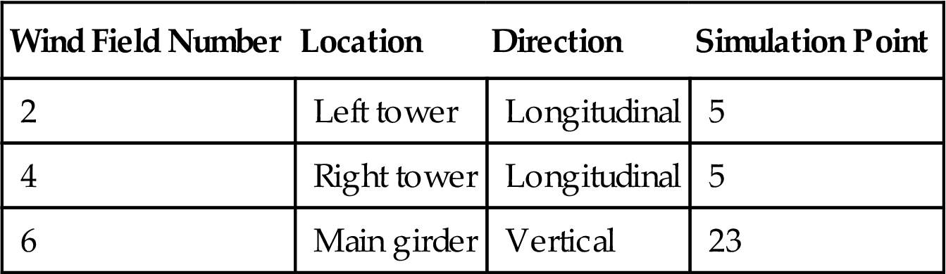
The wind field can be simplified into three independent one-dimension multivariable random wind velocity fields, as shown in Table 8.5. Twenty-three simulation points are distributed along the girder from the left to the right with a space of 10 m, 5 simulation points are distributed along the main tower from the bottom to the top with a space of 5 m, and the distribution of simulated points is shown in Fig. 8.8. According to the above theory, the wind velocity time history is obtained. Fig. 8.10 shows simulating results of point 1 and point 23.

8.2.3 Semiactive Control Strategy
In this example, the MR damper is installed in the cable-stayed bridge to control the longitudinal floating, the longitudinal displacement of the main tower, and the vertical bending displacement of the first mode of the bridge girder. According to the principle, the MR damper will be installed between the tower and the girder, as shown in Fig. 8.11, and the MR dampers are installed at points 48, 124, 192, and 286.

According to the previous intelligent control algorithm discussed in Chapter 2, Intelligent Control Strategies, the optimal control force of the MR damper can be calculated using the LQR optimal control algorithm. However, the MR damper cannot provide the calculated optimal control forces in any instant, thus the appropriate semiactive controlled strategy which fit the control of the bridge should be employed. Here, the idea of tristate control is adapted to adjust the inputting current, as seen in Eq. (8.6), which is similar to the semiactive controlled strategy discussed in Section 8.1.
(8.6)
 (8.6)
(8.6)
where ![]() and
and ![]() are the control forces of MR dampers with no current and the magnetic saturation current.
are the control forces of MR dampers with no current and the magnetic saturation current. ![]() is the displacement of the control point,
is the displacement of the control point, ![]() is the optimal control force,
is the optimal control force, ![]() and
and ![]() are the longitudinal optimal control forces of the control points 1 and 2, respectively, and
are the longitudinal optimal control forces of the control points 1 and 2, respectively, and ![]() is the installation angle, as shown in Fig. 8.11.
is the installation angle, as shown in Fig. 8.11.
The corresponding schematic diagram of the control strategy is shown in Fig. 8.12. The control forces are changing with the dynamic responses of each time through adjusting the input current.

8.2.4 Results and Analysis
Based on the above modeling and control strategy, the dynamic responses of the controlled and uncontrolled bridges are calculated. Fig. 8.13(A) shows the longitudinal displacement response of the bridge. The maximum longitudinal displacement responses are 141.5 mm for the uncontrolled bridge, 46.9 mm for the optimal controlled bridge with a reduction of 66.85%, and 71.0 mm for the tristate controlled bridge with a reduction of 49.82%. The tristate control strategy can effectively reduce the dynamic responses of longitudinal displacement responses of the bridge, although its control effect is inferior to the optimal control effect. Fig. 8.13(B) shows the acceleration responses of the bridge, it can be seen that the longitudinal acceleration responses are significantly reduced by using the MR damper. The acceleration peak value is 1.28 m/s2 for the uncontrolled bridge, 0.62 m/s2 for the controlled bridge with the tristate control strategy, and 0.42 m/s2 for the controlled bridge with the optimal control strategy.

The longitudinal displacement peak value of the main tower of the uncontrolled, the LQR optimal controlled, and the tristate controlled bridges are calculated, and the results are listed in Table 8.6. It can be seen that the displacement peak value is significantly reduced by using MR dampers. The peak value of the uncontrolled bridge is 132.8 mm, the peak value of the LQR optimal controlled bridge is 47.8 mm with a reduction of 64.01%, and the peak value of the tristate controlled bridge is 72.2 mm with a reduction of 45.63% compared with the uncontrolled bridge.
Table. 8.6
Peak vertical displacement of the of the tower under different control strategies
| Peak Displacement (m) | Uncontrolled and LOR Tristate Control | Uncontrolled and LOR Control | ||||
| Coordinate (x, y) | Uncontrolled | Tristate Control | Control Effect | Uncontrolled | Optimal Control | Control Effect |
| (−62.5, 30) | 0.1328 | 0.0722 | 45.63% | 0.1328 | 0.0478 | 64.01% |
| (−62.5, 25) | 0.1331 | 0.0734 | 44.85% | 0.1331 | 0.0505 | 62.06% |
| (−62.5, 20) | 0.1224 | 0.0682 | 44.28% | 0.1224 | 0.0480 | 60.78% |
| (−62.5, 15) | 0.0932 | 0.0523 | 43.88% | 0.0932 | 0.0375 | 59.76% |
| (−62.5, 10) | 0.0530 | 0.0299 | 43.58% | 0.0530 | 0.0216 | 59.25% |
| (−62.5, 5) | 0.0162 | 0.0092 | 43.21% | 0.0162 | 0.0067 | 58.64% |
| (−62.5, 0) | 0 | 0 | 0 | 0 | ||

Although the angle of the MR damper is relatively small to provide enough force to control the longitudinal displacement, the MR damper can also provide a vertical force to control the vertical displacement of the middle span node of the girder. The vertical displacement and acceleration responses of the middle span node are calculated and the results are shown in Fig. 8.14.

It can be seen from Fig. 8.14 that the peak value of vertical displacement responses of the middle span node is 88.5 mm for the uncontrolled bridge, and 80.7 mm for the LQR optimal controlled bridge with a reduction of 8.8%, and 59.5 mm for the LQR tristate controlled bridge with a reduction of 32.77%. The peak value of vertical acceleration responses of the middle span node is 0.8 m/s2 for the uncontrolled bridge, and 0.62 m/s2 for the LQR optimal controlled bridge with a reduction of 22.5%, and 0.46 m/s2 for the tristate controlled bridge with a reduction of 42.5%.
In order to show the control effect of the MR damper on the displacements of the main tower and girder, the peak values of sixteen points are extracted on the left main tower with an interval of 2 m, and the displacement envelop diagram of the left main tower is shown in Fig. 8.15. Similarly, the displacement envelop diagram of the girder is plotted by extracting the displacement of 46 points on the girder with an interval of 5 m, as shown in Fig. 8.16. It can be seen that the MR damper can significantly reduce the dynamic responses of the bridge structure.


8.3 Dynamic Analysis on Platform With MRE Devices
Many precision industrial and experimental processes cannot work accurately if the instruments are affected by external vibrations, since vibration sensitive components are used in modern mechanism, such as atomic force microscopes, space telescopes and interferometers. Generally, these precision equipment and optical instruments are usually placed on a platform, and the vibration energy will be transmitted to the instruments through the platform. Therefore, vibration suppression measures should be taken into account on platforms. In this section, dynamic response analysis of a platform structure with MRE devices will be introduced.
8.3.1 Modeling and Parameters
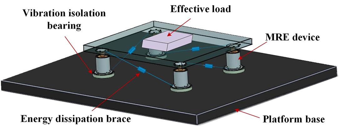
Fig. 8.17 shows the vibration isolation scheme of the platform system, which includes vibration isolation bearing, MRE device, and energy dissipation brace. The vibration isolation bearing is made of energy-guzzling viscoelastic material, which is used to isolate the excitation with high frequency and dissipate the input energy, so it is installed on the top of the platform base and connects to the MRE device. The energy dissipation brace is also made of energy-guzzling viscoelastic material, and installed between the two legs to resist the in-plane torsional vibrations of the platform. The stiffness and energy dissipation properties of the MRE devices can be adjusted according to the external excitation and structural responses, so as to mitigate the low frequency vibration.
Based on the vibration mitigation mechanism of the platform system, the mathematical model of vibration isolation control system is established, as shown in Fig. 8.18. Considering the working environment and the motion state of the platform, the vibration isolation and mitigation system of the platform is simplified to a model with seven degree of freedom.

Parameters are specified as follows:
![]() : the vertical displacement of platform centroid;
: the vertical displacement of platform centroid;
![]() : the angular displacement of pitching motion state of the platform;
: the angular displacement of pitching motion state of the platform;
![]() : the angular displacement of lateroversion motion state of the platform;
: the angular displacement of lateroversion motion state of the platform;
![]() ,
, ![]() ,
, ![]() ,
, ![]() : the vertical displacements of platform corners A, B, C, D;
: the vertical displacements of platform corners A, B, C, D;
![]() ,
, ![]() ,
, ![]() ,
, ![]() : the vertical displacements of the platform legs A, B, C, D;
: the vertical displacements of the platform legs A, B, C, D;
![]() : the effective mass of the platform;
: the effective mass of the platform;
![]() : the stiffness coefficient of MRE device;
: the stiffness coefficient of MRE device;
![]() ,
, ![]() ,
, ![]() ,
, ![]() : the magnetic forces of MRE devices;
: the magnetic forces of MRE devices;
![]() : the damping coefficient of MRE device;
: the damping coefficient of MRE device;
![]() ,
, ![]() : the vertical and horizontal stiffness coefficient of the vibration isolating bearing;
: the vertical and horizontal stiffness coefficient of the vibration isolating bearing;
![]() ,
, ![]() : the vertical and horizontal damping coefficient of the vibration isolating bearing;
: the vertical and horizontal damping coefficient of the vibration isolating bearing;
![]() ,
, ![]() : the stiffness and damping coefficient of the energy dissipation brace;
: the stiffness and damping coefficient of the energy dissipation brace;
Based on the mathematical model, the motion equation of the controlled platform structure can be expressed as
(8.7)
where ![]() , in which x1, x2, and x3 separately are the vertical, pitching motion, and side tumbling motion displacement responses, and x4, x5, x6, and x7 separately are the displacement responses of platform legs.
, in which x1, x2, and x3 separately are the vertical, pitching motion, and side tumbling motion displacement responses, and x4, x5, x6, and x7 separately are the displacement responses of platform legs. ![]() is the mass matrix of the control system.
is the mass matrix of the control system. ![]() and
and ![]() separately are the damping and stiffness matrixes.
separately are the damping and stiffness matrixes. ![]() is the position matrix of damper control force.
is the position matrix of damper control force. ![]() and
and ![]() separately are the exciting force and damper control force. Introducing state vector
separately are the exciting force and damper control force. Introducing state vector ![]() , the above equation can be expressed in the form of state-space equations.
, the above equation can be expressed in the form of state-space equations.
Combined with the features of the platform (mass and size) in this example, and on the basis of the preliminary analysis, the parameters of the platform structure control system are shown in Table 8.7.
Table 8.7
Parameters of the vibration control system of the platform
| Parameter | Meaning of Parameter | Value |
| ms | The effective mass of platform | 300 kg |
| md | The mass of platform legs | 30 kg |
| Ixx | The rotational inertia of the Y axis | |
| Iyy | The rotational inertia of the X axis | |
| Kv | The vertical stiffness coefficient of the vibration isolating bearing | 1.5×10⁶ N/m |
| Cv | The vertical damping coefficient of the vibration isolating bearing | |
| KE | The initial stiffness coefficient of MRE device | 1.3×10⁶ N/m |
| CE | The initial damping coefficient of MRE device | |
| Kb | The stiffness coefficient of the energy dissipation brace | 0.5×10⁶ N/m |
| Cb | The damping coefficient of the energy dissipation brace | |
| 2a | Long side size of the platform | 1.2 m |
| 2b | Short side size of the platform | 1.0 m |
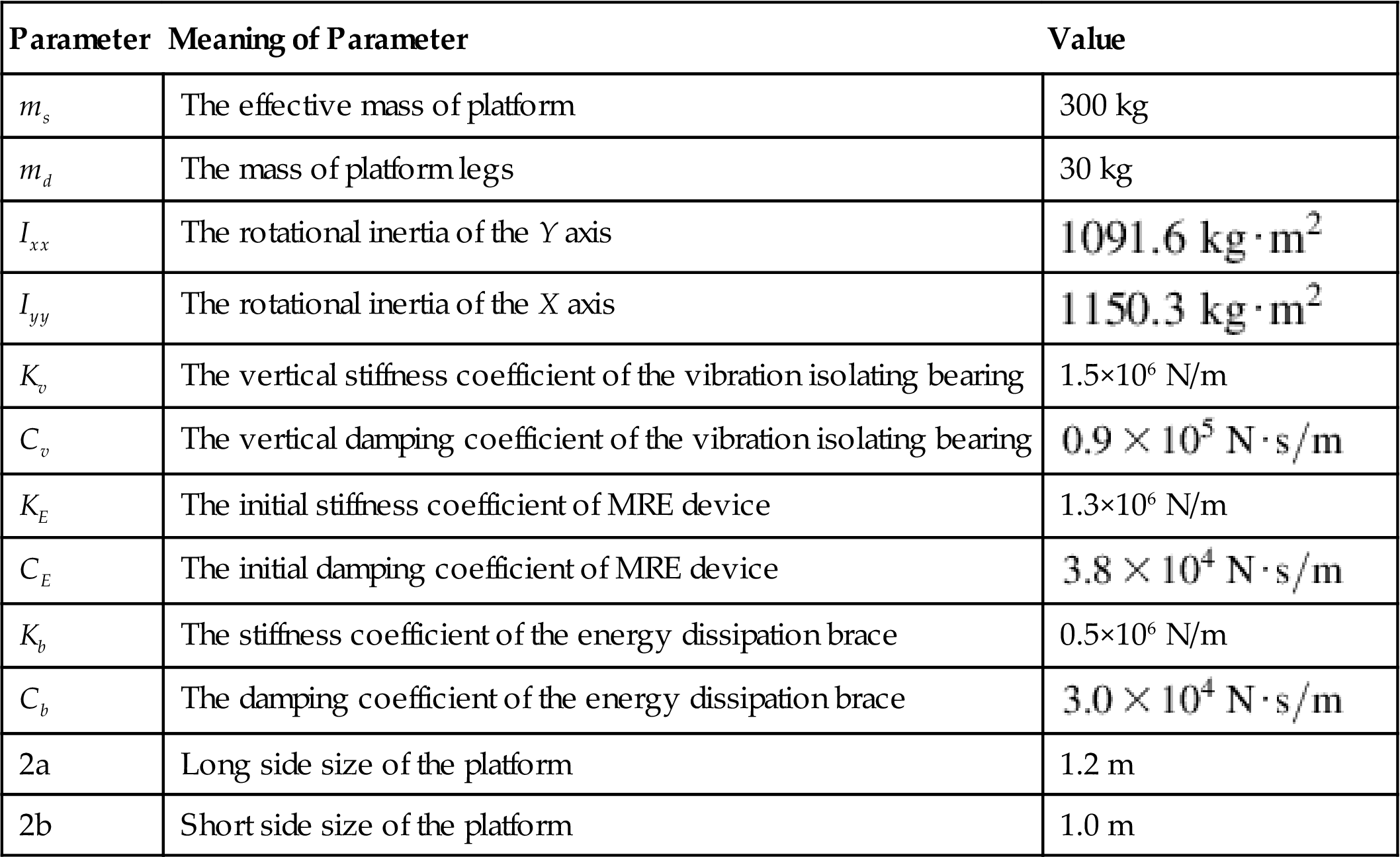
In Eq. (8.7), P(t) is a vector of the input excitation, which consists of the input excitations at the four supports of the platform. For structural dynamic analysis, the excitation data should be in the form of time-history input. In this example, the platform is thought to be rigid, so the time-history data of each input point (four supports of the platform) can be achieved from Eq. (8.8).
(8.8)
 (8.8)
(8.8)
8.3.2 Semiactive Control Strategy
For the platform structure with control devices, as shown in Fig. 8.17, when the parameters and excitation inputs of the motion equation are determined, dynamic analysis can be conducted by using MATLAB.
The optimal control force of the MRE device can be calculated using the LQR optimal control algorithm. However, the MRE device cannot provide the calculated optimal control forces in any instantaneous, thus an appropriate semiactive control strategy of the MRE device (Section 4.7) is designed, seen in Eq. (8.9).
(8.9)
 (8.9)
(8.9)
where ![]() is the vertical displacement absolute value of the platform centroid, a is the control target value of the platform centroid vertical displacement,
is the vertical displacement absolute value of the platform centroid, a is the control target value of the platform centroid vertical displacement, ![]() is the stroke of MRE device,
is the stroke of MRE device, ![]() is the thickness of MRE, and
is the thickness of MRE, and ![]() is an adjustment coefficient of the control current. When the vertical displacement response meets the control requirement, i.e.,
is an adjustment coefficient of the control current. When the vertical displacement response meets the control requirement, i.e., ![]() , the current value is 0. When the vertical displacement response cannot meet the control requirement and the maximum displacement response is less than the stroke of MRE device, the output force of MRE device can be controlled to close to the optimal control force by changing the current value. When the vertical displacement response is in the last state, the current value achieves as the maximum value.
, the current value is 0. When the vertical displacement response cannot meet the control requirement and the maximum displacement response is less than the stroke of MRE device, the output force of MRE device can be controlled to close to the optimal control force by changing the current value. When the vertical displacement response is in the last state, the current value achieves as the maximum value.
Based on the above control strategy, the current of MRE device needs to be chosen to realize the control effect, therefore the core idea for choosing current is dividing the work current into many states, and each state of working current corresponds with the output force value of MRE device. Fig. 8.19 shows the control strategy of the controlled platform structure, in which the response information about the controlled platform can be observed by sensors at any time, then the current is chosen according to the control law, which needs to be close to the optimal control force calculated by LQR method.

8.3.3 Results and Analysis
Based on the above modeling and control strategy, the dynamic responses of the controlled and uncontrolled platform structures are calculated. Fig. 8.20 shows the acceleration responses of the control system under passive control (the MRE device without current input, i.e., I=0). It can be seen that the acceleration responses of three directions under passive control obviously decreased. The power spectrum curves show that the dynamic responses of the passive controlled platform are reduced effectively compared to the uncontrolled platform when the excitation frequency is larger than 50 Hz, however, when the excitation frequency is in the scope of 0–10 Hz, the control effect is not obvious.

Table 8.8 shows the detail analysis results in frequency domain. It can be seen that when the frequency is in the scope of 30–50 Hz, the peak value of the power spectrum in Z direction, θy direction, and θx direction of the platform separately decreased from 1.51 m2/s4, 1.14 rad2/s4, and 1.37 rad2/s4 to 0.38 m2/s4, 0.11 rad2/s4 and 0.09 rad2/s4, respectively, and the corresponding reduction rates separately are 74.9%, 90.5%, and 93.4%. For the frequency 0–10 Hz, the reduction rates in three directions are −9.3%, 6.1%, and −11.8% separately, which means that the responses of the platform with passive control in the low frequency cannot be well controlled.
Table 8.8
Analysis results in frequency domain (passive control)
| Frequency | 0–10 Hz | 10–30 Hz | 30–50 Hz | |||||||
| Control Index | Z | θy | θx | Z | θy | θx | Z | θy | θx | |
| Uncontrol | Peak value | 1.21 | 1.49 | 1.28 | 1.17 | 1.50 | 1.27 | 1.51 | 1.14 | 1.37 |
| Passive control | Peak value | 1.32 | 1.4 | 1.43 | 1.11 | 0.75 | 0.72 | 0.38 | 0.11 | 0.09 |
| Reduction rate | −9.3% | 6.1% | −11.8% | 5.1% | 50% | 43.3% | 74.9% | 90.5% | 93.4% | |

Fig. 8.21 shows the analysis results of the semiactive controlled platform with the control strategy mentioned above, it can be seen that the acceleration responses in three directions are all well controlled, especially the peak value of acceleration power spectrum in low frequency (0–10 Hz). Compared to the passive control, the semiactive control with the appropriate control strategy can reach the better control effect in the whole spectrum (0–500 Hz).

Table 8.9 shows the detail analysis results in frequency domain. It can be seen that when the frequency is in the scope of 0–10 Hz, the peak value of the power spectrum in Z direction, θy direction, and θx direction of the platform separately decrease from 1.21 m2/s4, 1.49 rad2/s4, and 1.28 rad2/s4 to 0.75 m2/s4, 0.70 rad2/s4, and 0.78 rad2/s4, and the corresponding reduction rates separately are 38%, 53%, and 39.1%.
Table 8.9
Analysis results in frequency domain (semiactive control)
| Frequency | 0–10 Hz | 10–30 Hz | 30–50 Hz | |||||||
| Control Index | Z | θy | θx | Z | θy | θx | Z | θy | θx | |
| Uncontrol | Peak value | 1.21 | 1.49 | 1.28 | 1.17 | 1.50 | 1.27 | 1.51 | 1.14 | 1.37 |
| Semiactive control | Peak value | 0.75 | 0.70 | 0.78 | 0.57 | 0.45 | 0.34 | 0.13 | 0.08 | 0.05 |
| Reduction rate | 38.0% | 53.0% | 39.1% | 51.3% | 70.0% | 73.2% | 91.4% | 93.0% | 96.4% | |

8.4 SIMULINK Analysis Example
In Section 7.3, a simple example is used to introduce how the SIMULINK is operated. In this section, there are two SIMULINK examples to be introduced: one is a SIMULINK model of the structure without dampers, and the other is a SIMULINK model of the structure with MR dampers controlled by using the fuzzy controller and the neural network prediction model.
8.4.1 The SIMULINK Example of the Structure Without Dampers
In this example, a five-story steel frame structure without dampers is modeled and simulated by SIMULINK. The model story height vector is {h}={3.9, 3.3, 3.3, 3.3, 3.3}T m. The structural lumped mass matrix ![]() , the structural stiffness matrix
, the structural stiffness matrix ![]() , and the structural damping matrix
, and the structural damping matrix ![]() can be gained.
can be gained.


El Centro earthquake with 200 gal acceleration amplitude is selected, and the sampling time is 0.02 s. According to Eqs. (2.4) and (2.5), the state-space equation of the structure is given as:
(8.10)
 (8.10)
According to the Eq. (8.10), the SIMULINK model of the structure is built, as shown in Fig. 8.22. The “Xg” block is the input module of El Centro earthquake with 200 gal acceleration amplitude. The “[A]” block, “[D0]” block, “[E0]” block, and “{T}” block produce the system matrix ![]() , the input matrix
, the input matrix ![]() , the output matrix
, the output matrix ![]() , and the vector
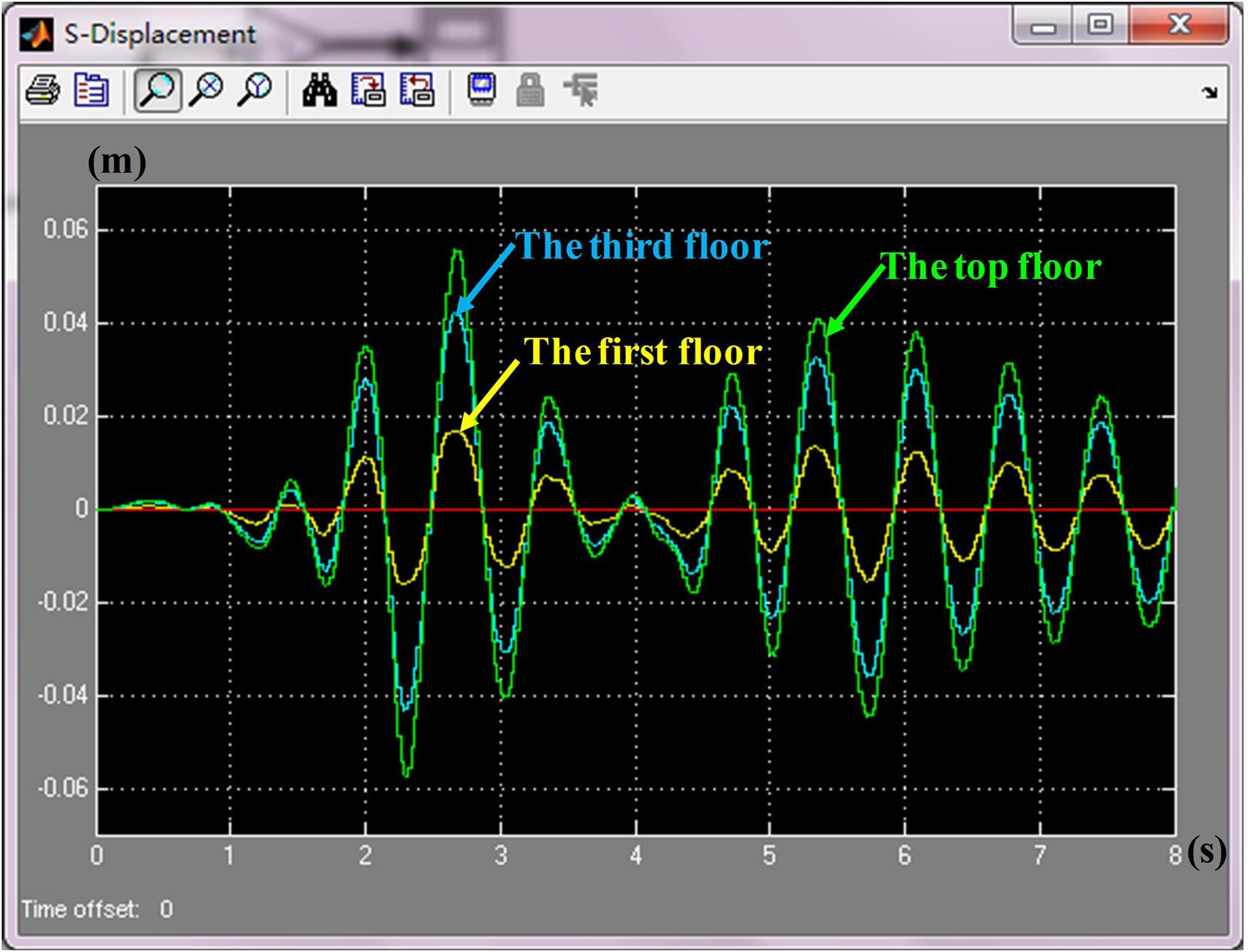
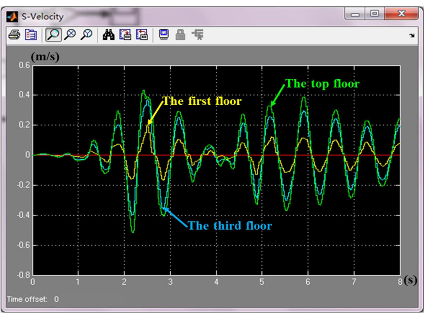
, and the vector ![]() , respectively. The “[E1]” block, “[E2],” and “[E3]” are the matrices to be used to extract the displacement, velocity, and acceleration responses of the first, third, and the top floors of the structure, respectively. There are four scopes, “E-Acceleration,” “S-Displacement,” “S-Velocity,” and “S-Acceleration,” to display the El Centro earthquake wave, the displacement, velocity, and acceleration responses of the first, third, and the top floors of the structure, respectively, as shown in Figs. 8.23–8.26. (Note: all units adopt the international system of units.)
, respectively. The “[E1]” block, “[E2],” and “[E3]” are the matrices to be used to extract the displacement, velocity, and acceleration responses of the first, third, and the top floors of the structure, respectively. There are four scopes, “E-Acceleration,” “S-Displacement,” “S-Velocity,” and “S-Acceleration,” to display the El Centro earthquake wave, the displacement, velocity, and acceleration responses of the first, third, and the top floors of the structure, respectively, as shown in Figs. 8.23–8.26. (Note: all units adopt the international system of units.)


8.4.2 The SIMULINK Example of the Controlled Structure
In this example, a five-story steel frame structure with two MR dampers placed in parallel in the first floor is simulated using SIMULINK, in which the structural parameters are the same as the model discussed in Section 8.4.1. The common MR dampers are adopted. The viscosity ![]() is 0.9 Pa·s. The effective length of the piston L is 400 mm, the gap Dh is 2 mm, and the inner diameter of the cylinder D is 100 mm. A fuzzy control strategy is proposed to produce the control currents of the MR damper, and a neuro network forecasting model of the steel frame structure is developed to predict the seismic responses of the structure with MR dampers, including the displacement and velocity responses of the first floor. El Centro earthquake with 200 gal acceleration amplitude is selected as the input excitation, and the sampling time is 0.02 s.
is 0.9 Pa·s. The effective length of the piston L is 400 mm, the gap Dh is 2 mm, and the inner diameter of the cylinder D is 100 mm. A fuzzy control strategy is proposed to produce the control currents of the MR damper, and a neuro network forecasting model of the steel frame structure is developed to predict the seismic responses of the structure with MR dampers, including the displacement and velocity responses of the first floor. El Centro earthquake with 200 gal acceleration amplitude is selected as the input excitation, and the sampling time is 0.02 s.
For frame structures, MR dampers are usually placed between the chevron braces as shown in Fig. 8.27, and the state-space equation of the controlled structure is given as Eq. (2.5). For the MR dampers, the most frequently referred Bingham model [197] is used to simulate the properties of the MR dampers, which includes a friction element in parallel to a viscous element as shown in Fig. 8.28, and a relation between the stress and strain rate is expressed as:
(8.11)
where ![]() is the shear stress in the fluid,
is the shear stress in the fluid, ![]() is the Newtonian viscosity which is independent of the applied magnetic field,
is the Newtonian viscosity which is independent of the applied magnetic field, ![]() is the shear strain rate and
is the shear strain rate and ![]() is the yield shear stress controlled by the applied magnetic field. Based on Eq. (8.11), Phillips [233] derived the force–displacement relationship for MR dampers:
is the yield shear stress controlled by the applied magnetic field. Based on Eq. (8.11), Phillips [233] derived the force–displacement relationship for MR dampers:
(8.12)
where ![]() is the frictional force,
is the frictional force, ![]() is the damping coefficient,
is the damping coefficient, ![]() is the length of the piston,
is the length of the piston, ![]() is the cross-sectional area of the piston,
is the cross-sectional area of the piston, ![]() is the inner diameter of the cylinder,
is the inner diameter of the cylinder, ![]() is the gap between the piston and the cylinder,
is the gap between the piston and the cylinder, ![]() is the relative displacement of the piston to the cylinder, and
is the relative displacement of the piston to the cylinder, and ![]() is the function of the applied magnetic field, which means
is the function of the applied magnetic field, which means ![]() is the function of control currents
is the function of control currents ![]() . Xu [249] proposed the relation between
. Xu [249] proposed the relation between ![]() and the control
and the control ![]() of the MR damper as follows:
of the MR damper as follows:
(8.13)
where ![]() ,
, ![]() , and
, and ![]() are coefficients relative to the property of the MR fluid in the MR damper, and
are coefficients relative to the property of the MR fluid in the MR damper, and ![]() is a constant.
is a constant.


A fuzzy controller is designed to control the working state of MR dampers. The two input variables are the earthquake acceleration excitation and the structural first floor displacement predicted by the neural network. The output variable is control current of MR dampers. The selection of the input variables of the fuzzy controller is based on the following two reasons: (1) The earthquake acceleration excitation influences on seismic responses of structures directly; (2) inter-story drifts are limited in seismic code, e.g., ![]() (
(![]() is the story height) is specified in the seismic code in China, so displacement responses are important parameters reflecting the control effects.
is the story height) is specified in the seismic code in China, so displacement responses are important parameters reflecting the control effects.
The basic domain of the earthquake acceleration is determined in accordance with the amplitude of the input acceleration. For an unknown earthquake wave beforehand, the basic domain can usually be determined as 0–10 m/s2, otherwise, the basic domain can be determined by the referenced range according to the limit of the magnitude of earthquake acceleration [250]. In this example, the 0.2 g El Centro earthquake wave is adopted as earthquake input, and then the basic domain is determined as 0–4 m/s2. The elastic limit of story drift is ![]() for frame structures according to the seismic code in China, where
for frame structures according to the seismic code in China, where ![]() is the story height. Therefore for the displacement response, the basic domain is 0–
is the story height. Therefore for the displacement response, the basic domain is 0–![]() . The basic domain of control currents of MR dampers is 0–2 A, same as the working current of MR dampers. According to basic domains of the earthquake acceleration excitation, the first floor displacement and control currents of MR dampers, fuzzy domains are determined as 0–4, 0–6 and 0–2, respectively. Accordingly, the corresponding quantification factors or proportion factors are determined as: the quantification factor of earthquake wave is
. The basic domain of control currents of MR dampers is 0–2 A, same as the working current of MR dampers. According to basic domains of the earthquake acceleration excitation, the first floor displacement and control currents of MR dampers, fuzzy domains are determined as 0–4, 0–6 and 0–2, respectively. Accordingly, the corresponding quantification factors or proportion factors are determined as: the quantification factor of earthquake wave is ![]() , the quantification factor of the first floor displacement of structure is
, the quantification factor of the first floor displacement of structure is ![]() , the proportion factor of control currents of MR dampers is
, the proportion factor of control currents of MR dampers is ![]() .
.
The earthquake acceleration, the structural first floor displacement and control currents of MR dampers may be divided into five grades, i.e., {VS (very small), S (small), M (middle), B (big), VB (very big)}, and their membership function curves are plotted in Fig. 8.29. Fuzzy rules of the fuzzy controller are listed in Table 8.10.

Table 8.10
Fuzzy rules of the fuzzy controller
| Displacement | Acceleration | ||||
| VS | S | M | B | VB | |
| VS | VS | VS | VS | VS | S |
| S | S | S | S | M | M |
| M | S | M | B | B | VB |
| B | S | B | B | VB | VB |
| VB | B | VB | VB | VB | VB |

A three-layer feed-forward neural network model is trained to predict structural dynamic responses to resolve the time-delay problem of the structure with MR dampers. The neural network model consists of an input layer, a hidden layer, and an output layer, as shown in Fig. 8.30. The input variables of the neural network are the ![]() th and
th and ![]() th time earthquake accelerations
th time earthquake accelerations ![]() , the
, the ![]() th and
th and ![]() th time control forces
th time control forces ![]() and the
and the ![]() th,
th, ![]() th, and kth time seismic response including the displacement and velocity of the first floor (
th, and kth time seismic response including the displacement and velocity of the first floor (![]() ,
, ![]() ,
, ![]() ,
, ![]() ,
, ![]() ,
, ![]() ). The output variables of the neural network are the next time-step displacement response of the first floor
). The output variables of the neural network are the next time-step displacement response of the first floor ![]() , and the next time-step velocity response of the first floor
, and the next time-step velocity response of the first floor ![]() . The predicted value
. The predicted value ![]() is one input variable of the fuzzy controller, and the predicted value
is one input variable of the fuzzy controller, and the predicted value ![]() is one of variables applied to gain control forces of MR dampers installed the first floor of the structure.
is one of variables applied to gain control forces of MR dampers installed the first floor of the structure.

Based on the analysis and design, the SIMULINK model of the intelligent control system of the controlled steel frame structure is built in accordance with the SIMULINK operations in Section 7.3, as shown in Fig. 8.31. The “NNET” block is the neural network forecasting model used to predict seismic responses of the structure with MR dampers, including the displacement and velocity of the first floor. The “fuzzy logic controller” block is the fuzzy controller used to produce controlled current of MR dampers. The “Ka” block produces the quantification factor of earthquake wave value, ![]() ; the “Kd” block produces the quantification factor of the displacement response of the first floor structure,
; the “Kd” block produces the quantification factor of the displacement response of the first floor structure, ![]() ; the “Kc” block produces the proportion factor of control currents of MR dampers value,
; the “Kc” block produces the proportion factor of control currents of MR dampers value, ![]() . The “MR damper” block is the subsystem simulating the nonlinear behavior of MR dampers, as shown in Fig. 8.32. The “E-Acceleration” block is an earthquake excitation source. The “E1” block is a matrix used to extract the first floor displacement from dynamic responses of the structure; the “C1” block is a matrix used to extract the first floor velocity from dynamic responses of the structure; the “C2” block is a matrix used to extract the predicted displacement of the first floor of the structure from the values predicted by the neural network forecasting model; the “C3” block is a matrix used to extract the predicted velocity of the first floor of the structure from the values predicted by the neural network forecasting model. The “S-Displacement” block displays displacement responses of the fuzzy control system.
. The “MR damper” block is the subsystem simulating the nonlinear behavior of MR dampers, as shown in Fig. 8.32. The “E-Acceleration” block is an earthquake excitation source. The “E1” block is a matrix used to extract the first floor displacement from dynamic responses of the structure; the “C1” block is a matrix used to extract the first floor velocity from dynamic responses of the structure; the “C2” block is a matrix used to extract the predicted displacement of the first floor of the structure from the values predicted by the neural network forecasting model; the “C3” block is a matrix used to extract the predicted velocity of the first floor of the structure from the values predicted by the neural network forecasting model. The “S-Displacement” block displays displacement responses of the fuzzy control system.


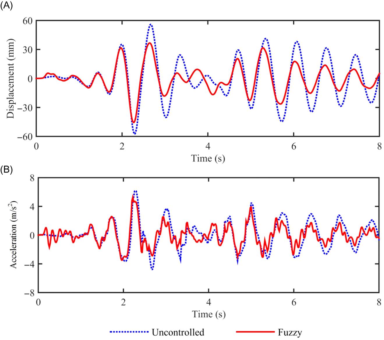
Fig. 8.33(A) and (B) shows the displacement and acceleration responses of the top floor of the fuzzy controlled and uncontrolled structures. It can be seen from Fig. 8.33 that both the displacement and acceleration responses of the fuzzy controlled structure are reduced effectively, especially for the displacement responses. The maximum displacement response of the top floor in the fuzzy controlled structure is 45.60 mm, by the reduction of 20.74% compared with that of the uncontrolled structure, 57.53 mm. At the same time, the maximum acceleration response of the top floor in the fuzzy controlled structure is 5.27 m/s2, by the reduction of 14.31% compared with that of the uncontrolled structure, 6.15 m/s2. Notice that, the seismic responses of the fuzzy controlled structure slightly increase at the early stage of the simulation. One contributing factor for this phenomenon is the deviation existing in the neural network forecasting model in the early simulation. The neural network is trained on line by collecting every time-step seismic responses of the structure with MR dampers, however, at the early stage, it is lack of training data. Hence, the predicted displacement and velocity responses are not accurate enough, and the error of the control force of MR dampers exists inevitably, which may result in the magnification of dynamic responses. Nevertheless, the magnification does not affect the control effect of the fuzzy control strategy due to that the period of magnified dynamic responses is very short.
For the sake of illuminating the efficiency of the fuzzy control strategy, the structural seismic responses under the fuzzy control strategy are compared with those under the passive-off and passive-on control strategy. The passive-off and passive-on control strategies belong to the passive mode, i.e., MR dampers are held at 0 A in the passive-off control strategy and the maximum current level (2 A) in the passive-on controlled strategy. Fig. 8.34(A) and (B) shows the displacement and acceleration responses of the top floor among the fuzzy controlled structure and the passive-off controlled structure. Fig. 8.35(A) and (B) shows the displacement and acceleration responses of the top floor of the fuzzy controlled structure and the passive-on controlled structure. It can be seen from Fig. 8.34 that the maximum displacement response of the top floor in the fuzzy controlled structure is 45.60 mm, by the reduction of 14.69% compared with that of the passive-off controlled structure, 53.45 mm. The maximum acceleration response of the top floor in the fuzzy controlled structure is 5.27 m/s2, by the reduction of 7.71% compared with that of the passive-off controlled structure, 5.71 m/s2. It is easy to comprehend that the control effect of the fuzzy control strategy is better than that of the passive-off control strategy, because control forces of MR dampers under the fuzzy control strategy are stronger and more appropriate than those under the passive-off control strategy. It can be seen from Fig. 8.35 that the maximum displacement response of the top floor in the fuzzy controlled structure is 45.60 mm, by the reduction of 8.19% compared with that of the passive-off controlled structure, 53.45 mm. The maximum acceleration response of the top floor in the fuzzy controlled structure is 5.27 m/s2, by the reduction of 22.39% compared with that of the passive-on controlled structure, 6.79 m/s2. Notice that the displacement responses under the fuzzy control strategy are slightly smaller than those under the passive-on control strategy; while the acceleration responses under the fuzzy control strategy are obviously smaller than those under the passive-on control strategy. The largest control forces produced by MR dampers usually donot benefit to control the acceleration under the passive-on control strategy. Nevertheless, the fuzzy control strategy can produce appropriate control forces to reduce the structural seismic responses. Apparently, choosing the passive-on strategy that produces the largest damping forces may not always be the most effective approach to protect the structure.


Compared with the commonly used bistate control strategy, how about the fuzzy control strategy? The bistate control strategy means that control currents of MR dampers can be turned on or off in real time. If the structure is moving away from its equilibrium position, control currents of MR dampers are turned on and reach the maximum value. If the structure is returning to its equilibrium position, control currents of MR dampers are turned off and reach the minimum value. In this study, the maximum working current of MR dampers is 2 A, and the minimum current is 0 A under the bistate control method. Fig. 8.36(A) and (B) shows the displacement and acceleration responses of the top floor of the fuzzy controlled structure and the bistate controlled structure. It can be shown that the maximum displacement response of the top floor in the fuzzy controlled structure is 45.60 mm, by the reduction of 16.76% compared with that of the bi-state controlled structure, 54.78 mm. The maximum acceleration response of the top floor in the fuzzy controlled structure is 5.27 m/s2, by the reduction of 30.84% compared with that of the bistate controlled structure, 7.62 m/s2. The numerical comparison results illustrate that the bistate control strategy is not an ideal control strategy although it is easy to realize. The main reason is that the bistate control strategy is a rough control strategy which cannot generate proper control currents of MR dampers. The fuzzy control strategy is a fine control strategy having the strong robustness and can determine appropriate control currents of MR dampers.

The maximum displacement and acceleration responses comparison of each floor under different control strategies are given in Fig. 8.37(A) and (B). It can be seen that the fuzzy control strategy is the most effective control strategy among the above control strategies. Since the passive-on control strategy adopts the maximum control currents of MR damper, its earthquake mitigation effect for the structural displacement response is good, especially for the maximum displacement responses of the second floor (20.74 mm) and the third floor (34.27 mm), which are smaller than those of the fuzzy control strategy (24.40 mm, 35.15 mm). However, the maximum acceleration responses under the passive-on control strategy are larger than those under the fuzzy control strategy due to the large control forces of MR dampers, which means providing the large equivalent stiffness to the structure. The maximum acceleration responses are increased due to the inappropriate currents of MR dampers under the bistate control strategy, moreover, the earthquake mitigation effect of the bistate control strategy for the structural displacement responses is also worse than that of the fuzzy control strategy. Obviously, the control effect of the fuzzy control strategy is better than the passive-on control strategy and the bistate control strategy as a whole, especially for the acceleration responses. For example, the maximum acceleration response of the second floor in the fuzzy controlled structure is 3.68 m/s2, by the reduction of 24.12% compared with that of the passive-on controlled structure, 4.85 m/s2, and by the reduction of 52.76% compared with that of the bistate controlled structure, 7.79 m/s2.

8.5 Particle Swarm Optimization Control Example
In this example, a five-story structure with five MR dampers (one MR damper is installed on each floor, as shown in Fig. 8.38) analyzed under the Particle Swarm Optimization (PSO) algorithm, the passive-on control algorithm, and the passive-off control algorithm, respectively.

8.5.1 Structural and Damper Parameters
The model structure is same as the model in Section 8.4.1. The common MR dampers are adopted. The MR fluids viscosity is 1.5 Pa·s. The effective length of the piston L is 844.3 mm, the inner diameter of the cylinder D is 203 mm, the piston cross-sectional area Ap is ![]() , and the gap h is 2.06 mm. El Centro earthquake with 200 gal acceleration amplitude is selected, and the sampling time is 0.02 s.
, and the gap h is 2.06 mm. El Centro earthquake with 200 gal acceleration amplitude is selected, and the sampling time is 0.02 s.
In the PSO optimization control of the frame structure with MR dampers, multiobjective optimization control method is adopted. The objective function is the combination of the displacement responses and the acceleration responses of the controlled structure, so the fitness function is obtained:
(8.14)
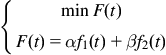 (8.14)
(8.15)
(8.16)
where ![]() and
and ![]() are the objective function of the displacement responses and the acceleration responses of the structure with MR dampers, respectively.
are the objective function of the displacement responses and the acceleration responses of the structure with MR dampers, respectively. ![]() and
and ![]() are the weight coefficients, and
are the weight coefficients, and ![]() . In this example,
. In this example, ![]() and
and ![]() .
. ![]() is the time variable.
is the time variable. ![]() and
and ![]() are the displacement response and the acceleration response of the nth floor of the structure, respectively.
are the displacement response and the acceleration response of the nth floor of the structure, respectively. ![]() and
and ![]() are the allowable maximum displacement response and acceleration response of the nth floor of the structure, respectively. According to the requirement of the building antiseismic design and building codes, when the structure is under the elastic state, the allowable maximum displacement response of the structure is
are the allowable maximum displacement response and acceleration response of the nth floor of the structure, respectively. According to the requirement of the building antiseismic design and building codes, when the structure is under the elastic state, the allowable maximum displacement response of the structure is ![]() (
(![]() is the story height of the structure); when the structure is under the elastoplastic state, the allowable maximum displacement response of the structure is
is the story height of the structure); when the structure is under the elastoplastic state, the allowable maximum displacement response of the structure is ![]() .
.
8.5.2 The PSO Optimization Control
In this example, the PSO algorithm with constriction factor is used to update the velocity and position of the particle, and the equations are shown as Eqs. (2.146) and (2.147). The parameters are ![]() ,
, ![]() ,
, ![]() . The particle swarm size is 30, and the number of the dimension in the problem space is 5.
. The particle swarm size is 30, and the number of the dimension in the problem space is 5.
In the PSO optimization control of the frame structure with MR dampers, the termination conditions of the PSO algorithm are the displacement and acceleration responses of the structure are less than the allowable value in the antiseismic design codes. That is, when the displacement and acceleration responses of the structure are less than the preset ![]() and
and ![]() , the optimization program will be terminated and the control current will be outputted.
, the optimization program will be terminated and the control current will be outputted.
8.5.3 Results and Analysis
For the sake of illuminating the efficiency of the PSO algorithm, the structure seismic responses under the PSO algorithm are compared with those of the uncontrolled, the passive-off and passive-on control structures. Fig. 8.39(A) and (B) shows the displacement and acceleration responses of the top floor of the PSO controlled structure and the uncontrolled structure. Fig. 8.40 (A) and (B) shows the displacement and acceleration responses of the top floor of the PSO controlled structure and the passive-off controlled structure. Fig. 8.41 (A) and (B) shows the displacement and acceleration responses of the top floor of the PSO controlled structure and the passive-on controlled structure.


It can be seen from Fig. 8.39 that the displacement responses of the PSO controlled structure are reduced effectively. The maximum displacement response of the top floor in the PSO controlled structure is 19.3 mm, by the reduction of 66.43%, compared with that of the uncontrolled structure, 57.5 mm. For the acceleration responses, the PSO algorithm can improve the earthquake mitigation effect slightly. The maximum acceleration response of the top floor in the PSO controlled structure is 5.90 m/s2, by the reduction of 10.58% compared with that of the uncontrolled structure, 6.60 m/s2.
As shown in Fig. 8.40, compared with the passive-off controlled structure, the displacement responses of the PSO controlled structure are reduced effectively. The maximum displacement response of the top floor in the PSO controlled structure is 19.3 mm, by the reduction of 63.03%, compared with that of the passive-off controlled structure, 52.2 mm. For the acceleration responses, the PSO control stratetgy is not better than the passive-off control strategy. The maximum acceleration response of the top floor in the PSO controlled structure is 5.90 m/s2, by the magnification of 2.63% compared with that of the passive-off controlled structure, 5.75 m/s2.
It can be seen from Fig. 8.41 that the PSO control algorithm is inferior to the passive-on control algorithm when the control objective is the displacement response. For the acceleration responses, the PSO controlled structure is much better than the passive-on controlled structure. The maximum acceleration response of the top floor in the PSO controlled structure is 5.90 m/s2, by the magnification of 17.11% compared with that of the passive-on controlled structure, 5.75 m/s2.
The maximum displacement and acceleration responses comparison of each floor under different control strategies are given in Fig. 8.42(A) and (B). It can be seen that the control effect of the maximum displacement response of each floor in the PSO controlled structure is inferior to that of passive-on controlled structure. Nevertheless, the control effect of structural displacement responses is significant, and the minimum reduction of the maximum displacement of each floor can reach 53.57% of the corresponding value of the uncontrolled structure, which meets the requirement of the building antiseismic design and building codes. For the maximum acceleration response of each floor, structural acceleration response increases under the passive-on control. This phenomenon can be explained that the working current of the MR damper is always the maximum current (2 A) for the passive-on controlled structure, which results in the increases of the structural stiffness unreasonably. The PSO control algorithm can reduce the maximum acceleration response of each floor effectively, this is because the PSO control algorithm adopts optimal control current as possible based on the fitness function and requirements real time. So, the displacement and acceleration responses of the structure can be controlled effectively.

8.6 Active Control Example
In this section, there is an active control example to be introduced. As mentioned in Chapter 3, Active Intelligent Control, active tendon system (ATS) is an effective and common way of active control. So, ATS is taken as an example to introduce the active control system.
8.6.1 Modeling and Parameters
In this example, a three-story frame structure is selected. The structural parameters of the model are the mass vector {m}={3, 3, 3}T×105 kg and the initial stiffness vector {k}={2, 2, 2}T×108 N/m. The damping matrix of the structure adopts Rayleigh damping in which the first and the second damping ratios are both assumed as 0.05. El Centro earthquake with 200 gal acceleration amplitude is selected as excitation, and the sampling time is 0.02 s. The dynamic responses of structures with and without ATS can be calculated by MATLAB programming.
According to the Eq. (3.20), the motion equation of the ATS control system can be expressed as Eq. (2.4). The mass matrix, the stiffness matrix, and the damping matrix of model can be expressed as follows:


and ![]() .
.
In this example, the active control devices are installed on each story of the structure, then the structure can be simplified, as shown in Fig. 8.43. Then the control force matrix and the position matrix can be expressed as
(8.17)
 (8.17)

As mentioned in Section 3.2, the state-space equation of the motion of ATS control system can be expressed as Eq. (2.5).
8.6.2 Active Control Strategy
In order to design an ATS, the active control force needs to be calculated firstly. LQR algorithm is the most widely used method in the design of the active control system, so the LQR optimal control algorithm is selected to design a state feedback controller fd(t), which makes the quadratic cost function minimum. Based on the explanation of the LQR algorithm in Section 2.2, this section mainly describes the steps to calculate the active control force by LQR algorithm.
Weight matrices [Q] and [R] are two vital control parameters in the LQR control algorithm, which determine the values of the control force and the structure response. The parameters [Q] and [R] can be expressed as:
(8.18)
where α and β are undetermined coefficients, [I] is a ![]() unit matrix.
unit matrix.
According to Section 3.2.3, the greater the [Q] is and the smaller the [R] is, then the smaller the structural responses and the greater of driving forces are. So in order to achieve better effect on active control, α is assumed as 100 and β is assumed as ![]() .
.
The state feedback gain matrix can be gained by the function lqr in MATLAB, as follows:
(8.19)
Then, according to Eq. (3.21) in the Section 3.3.2, the optimal driving force should be ![]() , and the state-space equation can be rewritten as the Eq. (3.22). Finally, the above equation can be solved by the function lsim in MATLAB:
, and the state-space equation can be rewritten as the Eq. (3.22). Finally, the above equation can be solved by the function lsim in MATLAB:
(8.20)
where ![]() is the unit matrix,
is the unit matrix, ![]() is the null matrix. The following program shows how to calculate the control force using the LQR algorithm in MATLAB:
is the null matrix. The following program shows how to calculate the control force using the LQR algorithm in MATLAB:
8.6.3 Results and Analysis
The maximum inter-story displacement and the maximum acceleration response are calculated in MATLAB, as shown in Table 8.11.
Table 8.11
| Condition | The Maximum Inter-Story Displacement (mm) | The Maximum Acceleration (m/s2) | ||||
| 1 | 2 | 3 | 1 | 2 | 3 | |
| Uncontrolled | 22.07 | 16.82 | 9.07 | 4.32 | 6.47 | 7.42 |
| ATS controlled | 2.68 | 1.78 | 0.90 | 1.29 | 1.83 | 2.03 |

It can be seen from Table 8.11 that the maximum inter-story displacement and the maximum acceleration can be reduced effectively by using active control. The maximum inter-story displacement of the first floor in the ATS controlled structure is 2.68 mm, by the reduction of 87.85%, compared with that of the uncontrolled structure, 22.07 mm. At the same time, the maximum acceleration response of the first floor in the ATS controlled structure is 1.29 m/s2, by the reduction of 70.14%, compared with that of the uncontrolled structure, 4.32 m/s2.
The time-history curve of the displacement response of the first floor is shown in Fig. 8.44. Similarly, the time-history curve of the acceleration responses of the first floor is shown in Fig. 8.45.


It can be seen that the displacement and the acceleration responses of the structure are reduced obviously by using the ATS control system. This also shows that the active control method has obviously vibration-suppressing effect when civil engineering structures are subjected to earthquake or strong wind excitations. However, the active control involves in many complex techniques, such as the strong power requirement, controller design, time-delay effect, therefore promotion and a lot of real applications of active control still require a period of time.