(2.79)

$\{Y_1(t)\}=\left[C_1\right]\{Z(t)\}+\left[B_1\right]\{f_d(t)\}$ (2.80)

(2.80)

$\{Y_2(t)\}=\left[C_2\right]\{Z(t)\}+\left[D_2\right]\{P(t)\}$ (2.81)

(2.81)

where $\{Z(t)\}$ is the state vector of system, $\{f_d(t)\}$ is the control input vector, $\{P(t)\}$ is the external input vector, $\{Y_1(t)\}$ and $\{Y_2(t)\}$ are the control output vector and the measured output vector, respectively, which are similar to the $\{Y(t)\}$ in Eq. (2.5). The design of controller mainly involves two aspects: one is the controller should make the system asymptotically stable, the other is to make the H_∞-norm of the sensitivity function (transfer function) minimum. The controller can be designed as the following:

$\{f_d(t)\}=-\left[G\right]\{Y_2(t)\}$ (2.82)

(2.82)

where $\left[G\right]$ is a gain matrix.

To obtain the transfer function matrix of the system, the measured output vector $\left\{Y_2\right\}$ is substituted into Eq. (2.82), then Eq. (2.82) is rewritten as:

$\{f_d(t)\}=-\left[G\right]\left[C_2\right]\{Z(t)\}-\left[G\right]\left[D_2\right]\{P(t)\}$ (2.83)

(2.83)

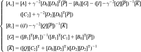
Substituting Eq. (2.83) into Eq. (2.79) and Eq. (2.80), the state-space equations of the controlled system and the controller can be written as:

$\{\stackrel{·}{Z}(t)\}=\left[\tilde{A}\right]\{Z(t)\}+\left[\tilde{B}\right]\{P(t)\}$ (2.84)

(2.84)

$\{Y_1(t)\}=\left[\tilde{C}\right]\{Z(t)\}+\left[\tilde{D}\right]\{P(t)\}$ (2.85)

(2.85)

where $\left[\tilde{A}\right]=\left[A\right]-\left[B_0\right]\left[G\right]\left[C_2\right]$, $\left[\tilde{B}\right]=-\left[B_0\right]\left[G\right]\left[D_2\right]+\left[D_0\right]$, $\left[\tilde{C}\right]=\left[C_1\right]-\left[B_1\right]\left[G\right]\left[C_2\right]$, $\left[\tilde{D}\right]=-\left[B_1\right]\left[G\right]\left[D_2\right]$. So, the transfer function matrix of system $\left[T_{Y_{1}P}\right]$ can be given by:

$\left[T_{Y_{1}P}\right]=\left[\tilde{C}\right]{([sI]-[\tilde{A}])}^{-1}\left[\tilde{B}\right]+\left[\tilde{D}\right]$ (2.86)

(2.86)

Thus the H_∞-norm of the transfer function matrix is defined as:

${\Vert T_{Y_{1}P}\Vert }_{\infty }=\underset{0\le w<\infty }{\sup }{\sigma }_{\max }[T_{Y_{1}P}(jw)]$ (2.87)

(2.87)

where ${\sigma }_{\max }[T_{Y_{1}P}(jw)]$ is the maximum singular value of the transfer function. For the single-input single-output system, the maximum singular value of the transfer function is the maximum modules amplitude of transfer function.

2.6.2 H_∞ Feedback Control

The infimum of the H_∞-norm set of the transfer function of controllers that ensure the closed-loop system stable is expressed as:

${\gamma }_{\infty }^{*}=\inf \left\{{\Vert T_{Y_{1}P}\Vert }_{\infty }|\mathrm{the}\mathrm{set}\mathrm{of}\mathrm{controllers}\mathrm{that}\mathrm{ensure}\mathrm{system}\mathrm{stable}\right\}$ (2.88)

(2.88)

If a controller can ensure the closed-loop system stable and ${\Vert T_{Y_{1}P}\Vert }_{\infty }<\gamma (\gamma >{\gamma }_{\infty }^{*})$, the controller is defined as ${\mathrm{H}}_{\infty }-\gamma$ suboptimal controller.

Generally, the measurements of all of the states of the controlled system are unrealizable, so the controller is designed based on the static output feedback approach. In any given case $\gamma >{\gamma }_{\infty }^{*}$, the controller can be designed as:

$\{\stackrel{·}{V}(t)\}=\left[A_c\right]\{V(t)\}+\left[B_c\right]\{Y_1(t)\}$ (2.89)

(2.89)

$\{f_d(t)\}=-\left[G\right]\{V(t)\}$ (2.90)

(2.90)

where $\{V(t)\}$ is the state vector of the controller.

$\{\begin{array}{ll}\left[A_c\right]& =\left[A\right]+{\gamma }^{-2}\left[D_0\right]{\left[D_0\right]}^{\mathrm{T}}\left[\overline{P}\right]-\left[B_0\right]\left[G\right]-{([I]-{\gamma }^{-2}[Q\left]\right[\overline{P}])}^{-1}\left[\overline{K}\right]\\ & ([C_2]+{\gamma }^{-2}[D_2\left]{\left[D_0\right]}^{\mathrm{T}}\right[\overline{P}])\\ \left[B_c\right]& ={((I)-{\gamma }^{-2}[Q\left]\right[\overline{P}])}^{-1}\left[\overline{K}\right]\\ \left[G\right]& ={({\left[B_1\right]}^{\mathrm{T}}[B_1])}^{-1}({\left[B_1\right]}^{\mathrm{T}}[C_1]+{\left[B_0\right]}^{\mathrm{T}}[\overline{P}])\\ \left[\overline{K}\right]& =([Q]{\left[C_2\right]}^{\mathrm{T}}+[D_0]{\left[D_2\right]}^{\mathrm{T}}){([D_2]{\left[D_2\right]}^{\mathrm{T}})}^{-1}\end{array}$ (2.91)

(2.91)

The matrixes $\left[\overline{P}\right]$ and $\left[Q\right]$ are the semi-positive definite solutions of the following Riccati matrix equations:

$\begin{array}{l}{\left[A\right]}^{\mathrm{T}}\left[\overline{P}\right]+\left[\overline{P}\right]\left[A\right]+{\left[C_1\right]}^{\mathrm{T}}\left[C_1\right]+\left[\overline{P}\right]\left[D_0\right]{\left[D_0\right]}^{\mathrm{T}}\left[\overline{P}\right]/{\gamma }^2\hfill \\ -([\overline{P}\left]\right[B_0]+{\left[C_1\right]}^{\mathrm{T}}[B_1]){({\left[B_1\right]}^{\mathrm{T}}[B_1])}^{-1}({\left[B_1\right]}^{\mathrm{T}}[C_1]+{\left[B_0\right]}^{\mathrm{T}}[\overline{P}])=0\hfill \end{array}$ (2.92)

(2.92)

$\begin{array}{l}\left[Q\right]{\left[A\right]}^{\mathrm{T}}+\left[A\right]\left[Q\right]+\left[D_0\right]{\left[D_0\right]}^{\mathrm{T}}+\left[Q\right]{\left[C_1\right]}^{\mathrm{T}}\left[C_1\right]\left[Q\right]/{\gamma }^2-\hfill \\ ([Q]{\left[C_2\right]}^{\mathrm{T}}+[D_0]{\left[D_2\right]}^{\mathrm{T}}){({\left[D_2\right]}^{\mathrm{T}}[D_2])}^{-1}([D_2]{\left[D_0\right]}^{\mathrm{T}}+[C_2\left]\right[Q])=0\hfill \end{array}$ (2.93)

(2.93)

Sometimes, the measurements of all of the states of the controlled system are realizable, so the control is designed based on the full state feedback approach, and the controlled system and the controller are expressed as:

$\{\stackrel{·}{Z}(t)\}=\left[A\right]\{Z(t)\}+\left[B_0\right]\{f_d(t)\}+\left[D_0\right]\{P(t)\}$ (2.94)

(2.94)

$\{Y_1(t)\}=\left[C_1\right]\{Z(t)\}+\left[B_1\right]\{f_d(t)\}$ (2.95)

(2.95)

$\{Y_2(t)\}=\{Z(t)\}$ (2.96)

(2.96)

The full state feedback controller is designed as:

$\{f_d(t)\}=-\left[G\right]\{Z(t)\}=-{({\left[B_1\right]}^{\mathrm{T}}[B_1])}^{-1}({\left[B_1\right]}^{\mathrm{T}}[C_1]+{\left[B_0\right]}^{\mathrm{T}}[\overline{P}])\{Z(t)\}$ (2.97)

(2.97)

where $\left[\overline{P}\right]$ is the positive-definite solution of the following Riccati equation:

$\begin{array}{l}{\left[A\right]}^{\mathrm{T}}\left[\overline{P}\right]+\left[\overline{P}\right]\left[A\right]+{\left[C_1\right]}^{\mathrm{T}}\left[C_1\right]+\left[\overline{P}\right]\left[D_0\right]{\left[D_0\right]}^{\mathrm{T}}\left[\overline{P}\right]/{\gamma }^2\hfill \\ -([\overline{P}\left]\right[B_0]+{\left[C_1\right]}^{\mathrm{T}}[B_1]){({\left[B_1\right]}^{\mathrm{T}}[B_1])}^{-1}({\left[B_1\right]}^{\mathrm{T}}[C_1]+{\left[B_0\right]}^{\mathrm{T}}[\overline{P}])=0\hfill \end{array}$ (2.98)

(2.98)

The excellent robustness is an advantage of ${\mathrm{H}}_{\infty }$ feedback control in the intelligent control of civil engineering structures. In addition, the operation of ${\mathrm{H}}_{\infty }$ feedback control is relatively simple, and the only problem is the selection of the transfer function matrix of the controlled structure.

2.7.1 Design of Sliding Surface

The equation of the linear time-invariant system can be expressed as Eq. (2.62), and the sliding surface can be designed as the linear combination of the state vectors of the system:

$\left\{S\right\}=\left[\mathrm{\Theta }\right]\{Z(t)\}$ (2.99)

(2.99)

where $\left[\mathrm{\Theta }\right]$ is a $p\times 2n$ matrix, which determines the stability and performance of the sliding mode, and the design of the sliding surface is to find the matrix $\left[\mathrm{\Theta }\right]$. The $\left[\mathrm{\Theta }\right]$ can be designed based on the LQR algorithm or the pole assignment algorithm, when the control is the full state feedback. If the static output feedback control is adopted, $\left[\mathrm{\Theta }\right]$ can be designed based on pole assignment algorithm. Here the LQR algorithm is selected to design the sliding surface.

Firstly, the state vector of the system is conducted by a linear transformation:

$\{y(t)\}=\left[T\right]\{Z(t)\}$ (2.100)

(2.100)

where $\left[T\right]$ is a state-transition matrix, which can be expressed as:

$\left[T\right]=\left[\begin{array}{cc}\left[I_{2n-p}\right]& -\left[B_1\right]{\left[B_2\right]}^{-1}\\ \left[0\right]& \left[I_p\right]\end{array}\right]$, ${\left[T\right]}^{-1}=\left[\begin{array}{cc}\left[I_{2n-p}\right]& \left[B_1\right]{\left[B_2\right]}^{-1}\\ \left[0\right]& \left[I_p\right]\end{array}\right]$, $\left[B_0\right]=\left[\begin{array}{c}\left[B_1\right]\\ \left[B_2\right]\end{array}\right]$; $\left[B_0\right]$ is the position matrix of installed controllers, which is rewritten as partition form, $(2n-p)\times p$ matrix $\left[B_1\right]$ and $p\times p$ matrix $\left[B_2\right]$. The former represents the position where controllers are not installed, the latter represents the position where p controllers are installed and is a nonsingular matrix. If the external load is ignored, the state equations of a system and sliding surface can be rewritten as:

$\{\stackrel{·}{y}(t)\}=\left[\tilde{A}\right]\{y(t)\}+\left[\tilde{B}\right]\{f_d(t)\}$ (2.101)

(2.101)

$\left[S\right]=\left[\tilde{\mathrm{\Theta }}\right]\{y(t)\}$ (2.102)

(2.102)

where $\left[\tilde{A}\right]=\left[T\right]\left[A\right]{\left[T\right]}^{-1}$, $\left[\tilde{B}\right]={[\begin{array}{cc}0& B_2^{\mathrm{T}}\end{array}]}^{\mathrm{T}}$, $\left[\tilde{\mathrm{\Theta }}\right]=\left[\mathrm{\Theta }\right]{\left[T\right]}^{-1}$. In order to achieve the feedback mechanism, the matrixes and vector in Eqs. (2.101) and (2.102) are rewritten as partition form: $\{y(t)\}={\{{\{y_1(t)\}}^{\mathrm{T}},{\{y_2(t)\}}^{\mathrm{T}}\}}^{\mathrm{T}}$, $\left[\tilde{A}\right]=\left[\begin{array}{cc}\left[{\tilde{A}}_{11}\right]& \left[{\tilde{A}}_{12}\right]\\ \left[{\tilde{A}}_{21}\right]& \left[{\tilde{A}}_{22}\right]\end{array}\right]$, $\left[\tilde{\mathrm{\Theta }}\right]=[\begin{array}{cc}\left[{\tilde{\mathrm{\Theta }}}_1\right]& \left[{\tilde{\mathrm{\Theta }}}_2\right]\end{array}]$.

Then the state equations of system and sliding surface can be expressed as:

$\{{\stackrel{·}{y}}_1(t)\}=\left[{\tilde{A}}_{11}\right]\{y_1(t)\}+\left[{\tilde{A}}_{12}\right]\{y_2(t)\}$ (2.103)

(2.103)

$\left\{S\right\}=\left[{\tilde{\mathrm{\Theta }}}_1\right]\{y_1(t)\}+\left[{\tilde{\mathrm{\Theta }}}_2\right]\{y_2(t)\}=0$ (2.104)

(2.104)

In order to simplify the derivation, the $\left[{\tilde{\mathrm{\Theta }}}_2\right]$ is assumed as a unit matrix, then:

$\{{\stackrel{·}{y}}_1(t)\}=([{\tilde{A}}_{11}]-[{\tilde{A}}_{12}\left]\right[{\tilde{\mathrm{\Theta }}}_1])\{y_1(t)\}$ (2.105)

(2.105)

$\{y_2(t)\}=-\left[{\tilde{\mathrm{\Theta }}}_1\right]\{y_1(t)\}$ (2.106)

(2.106)

Assuming that all of the states are measured, the performance index of the system is given by:

$J={\int }_{t_0}^{\infty }{\{Z(t)\}}^{\mathrm{T}}\left[Q\right]\{Z(t)\}\mathrm{d}t$ (2.107)

(2.107)

where $\left[Q\right]$ is a positive definite weighting matrix. The performance index of the system can be expressed by $\{y(t)\}$ after a further transformation:

$J={\int }_{t_0}^{\infty }{\{y(t)\}}^{\mathrm{T}}\left[\tilde{Q}\right]\{y(t)\}\mathrm{d}t$ (2.108)

(2.108)

where $\left[\tilde{Q}\right]={\left[T\right]}^{-1\mathrm{T}}\left[Q\right]{\left[T\right]}^{-1}=\left[\begin{array}{cc}\left[{\tilde{Q}}_{11}\right]& \left[{\tilde{Q}}_{12}\right]\\ \left[{\tilde{Q}}_{21}\right]& \left[{\tilde{Q}}_{22}\right]\end{array}\right]$.

In order to minimize the above performance index and satisfy the constraint, $\{y_2(t)\}$ is expressed by the feedback state $\{y_1(t)\}$ based on the maximum principle:

$\{y_2(t)\}=-0.5{\left[{\tilde{Q}}_{22}\right]}^{-1}({\left[{\tilde{A}}_{12}\right]}^{\mathrm{T}}[\tilde{P}]+2[{\tilde{Q}}_{21}])\{y_1(t)\}$ (2.109)

(2.109)

where $\left[\tilde{P}\right]$ is the solution of the following Riccati equation:

$\begin{array}{l}{\left[\hat{A}\right]}^{\mathrm{T}}\left[\tilde{P}\right]+\left[\tilde{P}\right]\left[\hat{A}\right]-0.5\left[\tilde{P}\right]\left[{\tilde{A}}_{12}\right]{\left[{\tilde{Q}}_{22}\right]}^{-1}{\left[{\tilde{A}}_{12}\right]}^{\mathrm{T}}\left[\tilde{P}\right]+\hfill \\ 2([{\tilde{Q}}_{11}]-[{\tilde{Q}}_{12}]{\left[{\tilde{Q}}_{22}\right]}^{-1}{\left[{\tilde{Q}}_{12}\right]}^{\mathrm{T}})=0\hfill \end{array}$ (2.110)

(2.110)

where $\left[\hat{A}\right]=\left[{\tilde{A}}_{11}\right]-\left[{\tilde{A}}_{12}\right]{\left[{\tilde{Q}}_{22}\right]}^{-1}\left[{\tilde{Q}}_{21}\right]$. So far, the sliding surface can be identified as

$\left[{\tilde{\mathrm{\Theta }}}_1\right]=-0.5{\left[{\tilde{Q}}_{22}\right]}^{-1}({\left[{\tilde{A}}_{12}\right]}^{\mathrm{T}}[\tilde{P}]+2[{\tilde{Q}}_{21}])$ (2.111)

(2.111)

$\left[\mathrm{\Theta }\right]=\left[\tilde{\mathrm{\Theta }}\right]\left[T\right]=\left[\right[{\tilde{\mathrm{\Theta }}}_1]⋮[I_p\left]\right]\left[T\right]$ (2.112)

(2.112)

2.7.2 Design of Controller

The design of the controller is the second phase of SMC design, and the aim is to make the state of the system tend to the sliding surface and keep stable on the surface. Here the controller is designed based on the Lyapunov direct method.

Setting Lyapunov function as follows:

$v=0.5{\left\{S\right\}}^{\mathrm{T}}\left\{S\right\}=0.5{\{Z(t)\}}^{\mathrm{T}}{\left[\mathrm{\Theta }\right]}^{\mathrm{T}}\left[\mathrm{\Theta }\right]\{Z(t)\}$ (2.113)

(2.113)

The sufficient condition to ensure the system performance stable on sliding surface is:

$\stackrel{·}{v}={\left\{S\right\}}^{\mathrm{T}}\left\{\stackrel{·}{S}\right\}\le 0$ (2.114)

(2.114)

Substituting Eq. (2.5) into Eq. (2.114), then

$\begin{array}{ll}\stackrel{·}{v}\hfill & ={\left\{S\right\}}^{\mathrm{T}}\left\{\stackrel{·}{S}\right\}={\left\{S\right\}}^{\mathrm{T}}\left[\mathrm{\Theta }\right]\{\stackrel{·}{Z}(t)\}={\left\{S\right\}}^{\mathrm{T}}\left[\mathrm{\Theta }\right]([A\left]\right\{Z(t)\}+[B_0\left]\right\{f_d(t)\}+[D_0\left]\right\{P(t)\})\hfill \\ \hfill & ={\left\{S\right\}}^{\mathrm{T}}\left[\mathrm{\Theta }\right]\left[B_0\right](\{f_d(t)\}+{([\mathrm{\Theta }\left]\right[B_0])}^{-1}[\mathrm{\Theta }](\left[A\right]\{Z(t)\}+\left[D_0\right]\{P(t)\}))\hfill \\ \hfill & =\left\{\lambda \right\}(\{f_d(t)\}-\{G_s\})=\sum _{i=1}^p{\lambda }_i(f_{di}-G_{is})\hfill \end{array}$ (2.115)

(2.115)

According to the above sufficient condition in Eq. (2.114), the control force derived from ith controller can be designed as

${f_{di}}^{*}(t)=\{\begin{array}{cc}{G}_{is}-W_i\mathrm{sgn}({\lambda }_i);& \mathrm{if}\sum _{i=1}^p-{\lambda }_i{G}_{is}\ge 0\\ 0;& \mathrm{if}\sum _{i=1}^p-{\lambda }_i{G}_{is}<0\end{array}$ (2.116)

(2.116)

where W_i is a given smaller constant, $W_i=(0.0001~0.0005)f_{d,\max }$. Considering the maximum driving force of the actuator, the final control force is given by:

$f_{di}(t)=\{\begin{array}{cc}{f_{di}}^{*}(t);& \mathrm{if}\left|{f_{di}}^{*}\right|<f_{d,\max }\\ f_{d,\max }\mathrm{sgn}({f_{di}}^{*}(t));& \mathrm{others}\end{array}$ (2.117)

(2.117)

The SMC is conducted by the above operation in civil engineering structures, in which the sliding surface can be defined as the linear combination of the state vectors of the controlled structure, and the controller can be designed through the Lyapunov direct method or the other control laws. Generally, the SMC is applied to the control that the parameters of the controlled system constantly change, such as the semi-active variable stiffness and variable damping controls.

2.8.1 Basic Principle

The physical stochastic optimal control is implemented by solving a collection of deterministic dynamic equations corresponding to the representative realizations with preassigned weights [47]. Hence it is spontaneous to develop a nonlinear stochastic optimal control strategy by integrating a physical stochastic control scheme and a deterministic nonlinear optimal control theory. According to the original physical scheme, the nonlinear stochastic optimal control strategy can be performed and optimized as follows [48]. Firstly, for each representative realization of stochastic parameters, the minimization of a cost function is executed to build a functional mapping from the set of parameters of control policy to the set of control gains. Then the specified parameters of control policy are obtained by minimizing a performance function related to the objective structural performance, as well as the corresponding control gain. The content mentioned above is the fundamental theory of stochastic optimal polynomial.

In Section 2.1, the motion equation of the structural system with a finite number n degrees of freedom under dynamic loads has been given as Eq. (2.1), which can be expressed as the following after mathematical simplification

$\left[M\right]\{\ddot{x}(t)\}+\left\{f\right[x(t),\stackrel{·}{x}(t)\left]\right\}=\left[B\right]\{f_d(t)\}+\left[D\right]\{F(\varpi ,t)\},$

$x(t_0)=x_0,\stackrel{·}{x}(t_0)={\stackrel{·}{x}}_0$ (2.118)

(2.118)

where $\{x(t)\}=\{x(\mathrm{\Theta },t)\}$ is an n-dimensional displacement vector; $\{f_d(t)\}=\{f_d(\mathrm{\Theta },t)\}$ is an r-dimensional control force vector; $\left[M\right]$ is a $n\times n$ mass matrix; $\left\{f\right[\text{∙}\left]\right\}$ is a n-dimensional vector denoting nonlinear internal forces, including a nonlinear damping force and a nonlinear restoring force; $\left\{F\right[\text{∙}\left]\right\}$ is a p-dimensional random excitation vector, in which $\varpi$ represents a point in the probability space, i.e., an embedded basic random event characterizing the randomness inherent in the external excitation. $\left\{\mathrm{\Theta }\right\}=\{\mathrm{\Theta }(\varpi )\}$ denotes a random parameter vector mapped from $\varpi$, which implicitly underlies the state and control force vectors. $\left[B\right]$ is a $n\times r$ matrix denoting the location of controllers; $\left[D\right]$ is a $n\times p$ matrix denoting the location of excitations.$x_0$ and ${\stackrel{·}{x}}_0$ are the initial displacement and initial velocity, respectively.

The classical OPC theory was proposed on the basis of Hamilton–Jacobi theoretical framework and the optimal principle [49], which is essentially the extended formulation of the LQR control in state space. In order to express Eq. (2.118) as the form of its state equation, the nonlinear internal force $\left\{f\right[\text{∙}\left]\right\}$ needs to be expanded. It is usually expressed as the following Maclaurin series:

$\begin{array}{ll}\left\{f\right[x(t),\stackrel{·}{x}(t)\left]\right\}\hfill & ={x\left\{\frac{\partial f[x,\stackrel{·}{x}]}{\partial x}+\frac{1}{2!}x\frac{{\partial }^{2}f[x,\stackrel{·}{x}]}{\partial x^2}+\cdots +\frac{1}{m!}{x}^{m-1}\frac{{\partial }^{m}f[x,\stackrel{·}{x}]}{\partial x^m}\right\}|}_{x=0,\stackrel{·}{x}=0}\hfill \\ \hfill & +{\stackrel{·}{x}\left\{\frac{\partial f[x,\stackrel{·}{x}]}{\partial \stackrel{·}{x}}+\frac{1}{2!}\stackrel{·}{x}\frac{{\partial }^{2}f[x,\stackrel{·}{x}]}{\partial {\stackrel{·}{x}}^2}+\cdots +\frac{1}{m!}{\stackrel{·}{x}}^{m-1}\frac{{\partial }^{m}f[x,\stackrel{·}{x}]}{\partial {\stackrel{·}{x}}^m}\right\}|}_{x=0,\stackrel{·}{x}=0}\hfill \end{array}$ (2.119)

(2.119)

where $m$ is the highest order of the Maclaurin series, and is equal to the order of the nonlinear internal force, indicating that the terms of series with $(m+1)$ and the higher-order parts are zero. Meanwhile, the zero order terms and the $x^i{\stackrel{·}{x}}^j$ cross terms which make little contribution to the nonlinear internal force of engineering structure are omitted.

The state-space equation has been given as Eq. (2.5), with the initial state $\{Z(t_0)\}=z_0$; $\{P(t)\}$ is same as $\{F(\varpi ,t)\}$; and $\left[A\right]$ can be expressed as the following after mathematical deformation:

$\left[A\right]=\left[\begin{array}{cc}\left[0\right]& \left[{\rm I}\right]\\ {-{\left[M\right]}^{-1}\sum _{i=1}^m\frac{x^{i-1}}{i!}\frac{{\partial }^{i}f[x,\stackrel{·}{x}]}{\partial x^i}|}_{x=0,\stackrel{·}{x}=0}& {-{\left[M\right]}^{-1}\sum _{i=1}^m\frac{{\stackrel{·}{x}}^{i-1}}{i!}\frac{{\partial }^{i}f[x,\stackrel{·}{x}]}{\partial {\stackrel{·}{x}}^i}|}_{x=0,\stackrel{·}{x}=0}\end{array}\right]$ (2.120)

(2.120)

A polynomial cost function, in stochastic case with $\left\{\mathrm{\Theta }\right\}$ [50], is given by

$\begin{array}{ll}{J}_1(\{Z\},\{f_d(t)\},\{\mathrm{\Theta }\},t)\hfill & =S(\{Z(t_f)\},t_f)+\frac{1}{2}{\int }_{t_0}^{t_f}\left[{\{Z(t)\}}^{\mathrm{T}}\right[Q_Z\left]\right\{Z(t)\}\\ & +{\{f_d(t)\}}^{\mathrm{T}}\left[R_f\right]\{f_d(t)\}+\{h(Z,t)\}]\mathrm{d}t\hfill \end{array}$ (2.121)

(2.121)

where $S(\{Z(t_f)\},t_f)$ is the terminal cost; $\{Z(t_f)\}$ is the terminal state; $t_0$ and $t_f$ are the start and terminal time, respectively; $\left[Q_Z\right]$ is a $2n\times 2n$ positive semi-definite matrix denoting state weighting; $\left[R_f\right]$ is a $r\times r$ positive-definite matrix denoting control weighting; $\{h(Z,t)\}$ is the higher-order term of the cost function whose order is higher than the quadratic term.

The minimization of the polynomial cost equation will result in the celebrated Hamilton–Jacobi–Bellman equation [51]:

$\frac{\partial \{V(Z,t)\}}{\partial t}=-\underset{f_d}{\min }\left[\right\{H(Z,f_d(t)\},\{V\prime (Z,t)\},\left\{\mathrm{\Theta }\right\},t)]$ (2.122)

(2.122)

where the optimal cost function $\{V(Z,t)\}$ satisfies all the properties of a Lyapunov function, considered as [51]

$\{V(Z,t)\}=\frac{1}{2}{\{Z(t)\}}^{\mathrm{T}}\widetilde{[P(t)]\{}Z(t)\}+\{g(Z,t)\}$ (2.123)

(2.123)

where $\widetilde{[P(t)}]$ is a $2n\times 2n$ Riccati matrix [48]; $\{g(Z,t)\}$ is a positive-definite multinomial in $\{Z(t)\}$. The Hamiltonian function $\{H(\text{∙})\}$ is defined by [50]

$\begin{array}{l}\{H(Z,f_d(t),V\text{'}(Z,t),\mathrm{\Theta },t)\}=\frac{1}{2}\left[{\{Z(t)\}}^{\mathrm{T}}\right[Q_Z\left]\right\{Z(t)\}+{\{f_d(t)\}}^{\mathrm{T}}[R_f\left]\right\{f_d(t)\}+\{h(Z,t)\left\}\right]\\ +{\{V\text{'}(Z,t)\}}^{\mathrm{T}}([A\left]\right\{Z(t)\}+[B_0\left]\right\{f_d(t)\})\end{array}$ (2.124)

(2.124)

The necessary condition for the minimization of the right-hand side of Eq. (2.122) is

$\frac{\partial \{H(Z,f_d(t),V\text{'}(Z,t),\mathrm{\Theta },t)\}}{\partial f_d}=0$ (2.125)

(2.125)

The optimal nonlinear controller is then given by

$\{f_d(t)\}=-{\left[R_f\right]}^{-1}{\left[B_0\right]}^{\mathrm{T}}\left[\widetilde{P(t)}\right]\{Z(t)\}-{\left[R_f\right]}^{-1}{\left[B_0\right]}^{\mathrm{T}}\{g\prime (Z,t)\}$ (2.126)

(2.126)

To express the controller Eq. (2.126) as an explicit function, $\{g(Z,t)\}$ is chosen as the following [50]

$\{g(Z,t)\}=\sum _{i=2}^k\frac{1}{i}{\left[{\{Z(t)\}}^{\mathrm{T}}\right[M_i(t)\left]\right\{Z(t)\left\}\right]}^i$ (2.127)

(2.127)

where $[M_i(t)]$, $i=2,3,\dots ,k$ are $2n\times 2n$ Lyapunov matrices [49].

Both $\widetilde{[P(t)}]$ and $[M_i(t)]$ are related to the gradient matrix $\left[A\right]$. Therefore the gain matrices of the polynomial controller cannot be calculated off-line. An approximate solution to the gain matrices is obtained by linearizing the gradient matrix $\left[A\right]$ at the initial equilibrium point $z_0$ [50], i.e., replacing $\left[A\right]$ into $\left[A_0\right]=\left[A\right]|z_0$. Furthermore, the Riccati matrix $\widetilde{[P(t)}]$ and the Lyapunov matrices $[M_i(t)]$, for a class of optimal control system with time infinite, could be approximately evaluated as constant matrices ($\left[\tilde{P}\right]$ and $\left[M_i\right]$) by solving the following algebraic Riccati and Lyapunov equations, i.e., the steady-state Riccati and Lyapunov matrix equations, respectively

$\widetilde{[P}\left]\right[A_0]+{\left[A_0\right]}^{\mathrm{T}}\widetilde{[P}]-\widetilde{[P}\left]\right[B_0\left]{\left[R_f\right]}^{-1}{\left[B_0\right]}^{\mathrm{T}}\right[\tilde{P}]+[Q_Z]=0$ (2.128)

(2.128)

$\left[M_i\right]([A_0]-[B_0\left]{\left[R_f\right]}^{-1}{\left[B_0\right]}^{\mathrm{T}}\right[\tilde{P}])+{([A_0]-[B_0\left]{\left[R_f\right]}^{-1}{\left[B_0\right]}^{\mathrm{T}}\right[\tilde{P}])}^{\mathrm{T}}\left[M_i\right]+\left[Q_{Z,i}\right]=0$ (2.129)

(2.129)

where $i=2,3,\dots ,k$.

Eqs. (2.128) and (2.129) can be solved using any well-known numerical algorithms or by virtue of computing software, e.g., MATLAB.

Hence an optimal polynomial controller can be obtained analytically in the form

$\{f_d(t)\}=-{\left[R_f\right]}^{-1}{\left[B_0\right]}^{\mathrm{T}}\widetilde{\left[P\right]}\{Z(t)\}-{\left[R_f\right]}^{-1}{\left[B_0\right]}^{\mathrm{T}}\sum _{i=2}^k{\left[\right\{Z^{\mathrm{T}}(t)\left\}\right[M_i(t)\left]\right\{Z(t)\left\}\right]}^{i-1}\left[M_i\right]\{Z(t)\}$ (2.130)

(2.130)

Eq. (2.130) indicates that the polynomial controller consists of two components, the linear term which is the first order and the nonlinear term which is the odd higher order.

2.8.2 Applications

As an extended conventional LQR, OPC provides more flexibility in the control design and further enhances system performance. Under strong earthquakes, the main objective of intelligent control is to reduce the peak (maximum) response of the structure in order to minimize the damage. For both linear and nonlinear or hysteretic structures, it has been shown that the polynomial controller is more effective than the classical linear controller in suppressing the peak response, due to its ability to provide large control force under strong earthquakes [50,52].

At present, the optimal polynomial controller is widely applied in the control of highly nonlinear or inelastic hybrid protective systems, such as the base-isolated building using lead-core rubber bearings and the fixed-base yielded building. The performances of the optimal polynomial controller with respect to various control objectives are investigated by means of numerical simulations [50]. The results have shown obvious advantages of the optimal polynomial controller in the field of structural vibration control.

2.9.1 Basic Principle

The core of fuzzy control method is the fuzzy controller. The fuzzy controller mainly includes three parts: fuzzification, fuzzy reasoning, and defuzzification, and its basic structure is shown in Fig. 2.3.

A fuzzification of mathematical concepts is based on a generalization of these concepts from characteristic functions to membership functions. That is, fuzzification of accurate input values means the external excitation acquired by computer sampling is translated into the membership functions. The purpose of fuzzification is to change the variable type such that it can be accepted and operated by the knowledge base.

The formation and reasoning of fuzzy rules are based on the control rules which are designed by the experienced operator or expert. A fuzzy output set is obtained by fuzzy reasoning, namely a new fuzzy membership function. The purpose of fuzzy reasoning is to adapt the control rules, determine the fitness of each control rules, and then the outputs are gained by fuzzy rules weighted.

The output value can be obtained by defuzzification according to the output fuzzy membership function, and different methods can be used to find a representative accurate value as the control value. The purpose of defuzzification is to obtain the accurate output value, which can be applied to the actuator to realize control.

2.9.2 Design of Fuzzy Controller

The design of fuzzy controller mainly consists of the following parts.

2.9.2.2 Fuzzification of the accurate value

For the fuzzy controller, the input and output values must be fuzzy values. However, the input and output values of the actual controlled systems all are accurate values. Thus the fuzzification method should be employed to transform the accurate value to the fuzzy values. This process can be divided into two steps, the first step is to determine the fuzzy domain, and the second step is fuzzification.

The following formula can be adopted to transform the basic domain into the fuzzy fiedomain,

$y=\frac{2n}{b-a}\left[x-\frac{a+b}{2}\right]$ (2.131)

(2.131)

where $x$ and $y$ are accurate variable and fuzzy variable, respectively; $[a,b]$ is the basic domain of $x$; $[-n,+n]$ is the fuzzy domain of $y$; and $n$ is a positive integer which is larger than 2. In fact, Mamdani method often is used, i.e., $n=6$. In addition, then variable $x$ in the domain $[a,b]$ also can be transformed into the asymmetric domain $[-n,+m]$, where $n$ and $m$ are both positive integers which are larger than 2. The transformation formula is as follows:

$y=\frac{m+n}{b-a}\left[x-\frac{a+b}{2}\right]$ (2.132)

(2.132)

Fuzzification is to divide the continuous quantity in fuzzy domain into several levels, according to the requirement, each level can be regarded as a fuzzy variable and corresponds to a fuzzy subset or a membership function. Usually, the fuzzy domain can be divided into the following the fuzzy subsets described as language variable: [NB (negative big), NM (negative middle), NS (negative small), Z (zero), PS (positive small), PM (positive middle), PB (positive big)], respectively.

2.9.2.6 Defuzzification

The results of fuzzy reasoning are fuzzy set or membership functions, and they reflect the combination of different control languages. However, the controlled objective can only accept one control accurate quantity, thus one control accurate quantity should be chosen from the output fuzzy set. In other word, the method of defuzzification is to deduce a mapping from fuzzy set to the ordinary number set. The commonly used method are the coefficient weighted mean method, the gravity method, and the maximum membership degree method. These methods will be introduced as follows:

1. The coefficient weighted mean method
The output quantity of this method can be expressed as,

$u=\sum k_i\cdot x_i/\sum k_i$ (2.133)

(2.133)

where $u$ is the output value of solving fuzzy, $x_i$ is the fuzzy input, $k_i$ is the coefficient; the selection of $k_i$ should depend on the actual condition, and different coefficients will result in different response characteristics.

2. The gravity method
The gravity method means, that the gravity of the area enveloped by the fuzzy membership function curve and the output value is chosen as the abscissa. The following equation can be employed,

$u={\displaystyle \frac{\int x{\mu }_N(x)\mathrm{d}x}{\int {\mu }_N(x)\mathrm{d}x}}$ (2.134)

(2.134)

where $x$ is the fuzzy input, and ${\mu }_N(x)$ is the membership degree function. In the actual calculation process, the following simple equation is adopted,

$u=\sum x_i\cdot {\mu }_N(x_i)/\sum {\mu }_N(x_i)$ (2.135)

(2.135)

In addition, the gravity method is the special case of the coefficient weighted mean method, and they are same when $k_i={\mu }_N(x_i)$.

3. The maximum membership degree method

The maximum membership degree method is one of the simplest methods, and only the element with the maximum membership degree is chosen as the output value. What is more, the curve of the membership function should be convex (unimodal curve). If the curve is flat trapezoid, the element with a maximum membership degree is larger than 1 and the average value should be adopted.

2.10.1 Basic Principle

The neural network is proposed by studying the human information according to the modern neurobiology and understanding science. It can be seen as a network which is composed of a large number of interconnected neurons (processing unit). The neural work has the characteristics of strong adaptability, learning ability, nonlinear mapping ability, robustness, and fault tolerance.

The neurons can transmit information, and their models can be classified as three parts: threshold unit, linear unit, and nonlinear unit. Once the model of neuron is determined, the performance and ability of a neural network will mainly depend on the topological structure and the learning method. The topological structures of neural networks are usually divided as

2.10.2 Learning Method

Once the topological structure of the neural network is determined, the learning method is indispensable to attribute the network with an intelligent characteristic, which is also the core problem in intelligent control using the neural network method. Through learning, neural networks can grasp the characteristics of intelligent or nonlinear structures. The learning method is actually the adjusting method of the weight of network connection. There are three major learning paradigms, each corresponding to a particular abstract learning task. These are supervised learning, unsupervised learning, and reinforcement learning. When the supervised learning model is used, the output of the network and the desired output signal (i.e., supervised signals) are compared, and then according to the difference the network's weights will be adjusted, finally differences will be smaller. When the unsupervised learning model is used, after the input signals are sent into the network, according to the present rules (such as competition rules), the network’s weights will be adjusted automatically, and the network will have pattern classification function eventually. The reinforcement learning method is a kind of learning method between the above two. There are several basic learning methods such as Hebb learning the rules, Delta (δ) learning rules, Probability learning rules, Competition learning rules and Levenberg–Marquart algorithm, and so on. As an example of learning methods, the commonly used Levenberg–Marquart algorithm will be introduced in the following.

Levenberg–Marquart algorithm belongs to the supervised learning model. When the output value $\hat{y}$ is not equal with the expected output $y$, the error signal will propagate from the output end in the reverse direction of the net, and the weight and threshold values are always modified to make the output value close to the desired output. When sample $p(p=1,2,\dots ,P)$ is weight adjusted, it will be delivered to the other sample models for learning train until $P$ times are completed.

The quadratic error function of the input and output modes of each sample $P$ is defined as,

$E_p=\frac{1}{2}\sum _{l=1}^L{[y_p(l)-{\hat{y}}_p(l)]}^2=\frac{1}{2}\sum _{l=1}^L{e}_l^2$ (2.136)

(2.136)

Thus the error function of the whole system is,

$E=\frac{1}{2}\sum _{p=1}^P\sum _{l=1}^L{[y_p(l)-{\hat{y}}_p(l)]}^2=\sum _{p=1}^P{E}_p$ (2.137)

(2.137)

For simplicity, the subscript $p$ is omitted in the following equations, and the PIF is chosen as the error function of the system, thus

$E=\frac{1}{2}\sum _{l=1}^L{[y(l)-\hat{y}(l)]}^2=\frac{1}{2}\sum _{l=1}^L{e}_l^2$ (2.138)

(2.138)

where $L$ is the number of the output neuron, $e_l$ is the error of the $l\mathrm{th}$ output neuron.

The weighting adjustment should be proceeded in the reverse direction of the gradient of function $E$ to make the output close to the desired value as far as possible. When Levenberg–Marquardt algorithm is employed in the training process of feedback neural network, the weighting matrix can be expressed as [53]

$\left[{\mathit{w}}^{i+1}\right]=\left[{\mathit{w}}^i\right]-{\left[\frac{{\partial }^{2}E}{\partial {\mathit{w}}^{i2}}+\mu \left[\mathit{I}\right]\right]}^{-1}\left[\frac{\partial E}{\partial {\mathit{w}}^i}\right]$ (2.139)

(2.139)

where $i$ is the training steps, $\left[\partial E/\partial {\mathit{w}}^i\right]$ is the descent gradient of the performance function $E$ with respect to the weighting matrix $\left[{\mathit{w}}^i\right]$, $\mu (\mu \ge 0)$ is the control factor, $\left[\mathit{I}\right]$ is the unit matrix, and the Jacobi matrix of the weighting value can be obtained by the Taylor series expansion of the error vector $\left[\mathit{e}\right]([\mathit{e}]={[e_1,e_2,\dots ,e_L]}^{\mathrm{T}})$,

$\left[{\mathit{J}}^i\right]={\left[\begin{array}{cccc}{\displaystyle \frac{\partial e_1}{\partial w_1^i}}& {\displaystyle \frac{\partial e_1}{\partial w_2^i}}& \cdots & {\displaystyle \frac{\partial e_1}{\partial w_B^i}}\\ {\displaystyle \frac{\partial e_2}{\partial w_1^i}}& {\displaystyle \frac{\partial e_2}{\partial w_2^i}}& \cdots & {\displaystyle \frac{\partial e_2}{\partial w_B^i}}\\ ⋮& ⋮& \ddots & ⋮\\ {\displaystyle \frac{\partial e_L}{\partial w_1^i}}& {\displaystyle \frac{\partial e_L}{\partial w_2^i}}& \cdots & {\displaystyle \frac{\partial e_L}{\partial w_B^i}}\end{array}\right]}_{L\times B}$ (2.140)

(2.140)

where $L$ is the number of output neuron, and $B$ is number of weighting value. Combining Eqs. (2.139) and (2.140) can obtain the following equation,

$\left[{\mathit{w}}^{i\mathit{+}1}\right]=\left[{\mathit{w}}^{\mathit{i}}\right]-{\left[{\left[{\mathit{J}}^{\mathit{i}}\right]}^{\mathrm{T}}\right[{\mathit{J}}^{\mathit{i}}]+\mathit{\mu }[\mathit{I}\left]\right]}^{-1}{\left[{\mathit{J}}^{\mathit{i}}\right]}^{\mathrm{T}}\left[\mathit{e}\right]$ (2.141)

(2.141)

Eq. (2.141) is the key equation of Levenberg–Marquardt algorithm. The application of intelligent control on civil engineering structures by using Levenberg–Marquardt algorithm and neural network can be seen in the study [54].

2.11.1 Basic Principle

In 1995, based on the idea of a bird flock foraging, James Kennedy, American social psychologist, and Russell Eberhart, electrical engineer, proposed the PSO algorithm [55–59]. That is, the birds in the bird flock are abstracted as “particles” without mass and volume, and these “particles” will mutually collaborate and share information to update their current movement velocity and direction according to their own and swarm’s best historical movement state information. This kind of method can well coordinate the movement relationship between the particles themselves and swarm, and look for the optimal solution in the complex solution space. The following, the basic PSO algorithm and the improved PSO algorithms will be described.

2.11.1.1 The basic PSO algorithm

Assuming that,

${\mathbf{x}}_i=(x_{i1},x_{i2},\cdots x_{in})$ is the current position of the $i\mathrm{th}$ particle;

${\mathbf{v}}_i=(v_{i1},v_{i2},\cdots v_{in})$ is the current velocity of the $i\mathrm{th}$ particle;

${\mathbf{p}}_i=(p_{i1},p_{i2},\cdots p_{in})$ is the optimal position once experienced of the $i\mathrm{th}$ particle, and the optimal position stands for the optimal adaptive value. For the minimization problem, the smaller the objective value is, the better adaptive value is;

${\mathbf{p}}_g=(p_{g1},p_{g2},\cdots p_{gn})$ is the optimal location of all particles of the swarm that experienced.

The evolution equation of the basic PSO equation can be described as:

$v_{ij}(t+1)=v_{ij}(t)+c_1*ran{d}_1()*(p_{ij}(t)-x_{ij}(t))+c_2*ran{d}_2()*(p_{gj}(t)-x_{ij}(t))$ (2.142)

(2.142)

$x_{ij}(t+1)=x_{ij}(t)+v_{ij}(t+1)$ (2.143)

(2.143)

where subscript $j$ denotes the $j$ dimension of the particles, subscript $i$ denotes the $i\mathrm{th}$ particle of the swarm, $t$ is the generation, $c_1$ is the cognitive learning coefficient, $c_2$ is the social learning coefficient, and $ran{d}_1()$ and $ran{d}_2()$ are the dependent random value within the range of $[0,1]$.

There are three parts in Eq. (2.142). The first part is the former velocity of the particle, which makes the algorithm have the capability of global research. The second part (cognition part) means the process of the particle’s absorption of their own experience. The third part (social part) means the process of the particle absorption of the other particle. The model without the second part is called the social-only model, which converges quickly and may stick in the local optimal value for the complex problem. The model without the third part is called the cognition-only model, which cannot obtain the optimal value due to no contact between the individuals.