Chapter 6

Lighting

Figure 6.1 shows how important lighting and shading are in conveying the solid form and volume of an object. The unlit sphere on the left looks like a flat 2D circle, whereas the lit sphere on the right does look 3D. In fact, our visual perception of the world depends on light and its interaction with materials, and consequently, much of the problem of generating photorealistic scenes has to do with physically accurate lighting models.

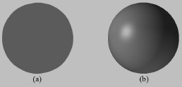
Figure 6.1: (a) An unlit sphere looks 2D. (b) A lit sphere looks 3D.

Of course, in general, the more accurate the model, the more computationally expensive it is; thus a balance must be reached between realism and speed. For example, 3D special FX scenes for films can be much more complex and utilize more realistic lighting models than games because the frames for a film are pre-rendered, so they can afford to take hours or days to process a frame. Games, on the other hand, are real-time applications, and therefore, the frames need to be drawn at a rate of at least 30 frames per second.

Note that the lighting model explained and implemented in this book is largely based on the one described in [Möller02].

Objectives:

    To gain a basic understanding of the interaction between lights and materials.

    To understand the differences between local illumination and global illumination.

    To find out how we can mathematically describe the direction a point on a surface is “facing” so that we can determine the angle at which incoming light strikes the surface.

    To learn how to correctly transform normal vectors.

    To be able to distinguish between ambient, diffuse, and specular light.

    To learn how to implement directional lights, point lights, and spotlights.

    To understand how to vary light intensity as a function of depth by controlling attenuation parameters.

6.1 Light and Material Interaction

When using lighting, we no longer specify vertex colors directly; rather, we specify materials and lights, and then apply a lighting equation, which computes the vertex colors for us based on light/material interaction. This leads to a much more realistic coloring of the object (compare the spheres in Figure 6.1 again).

Materials can be thought of as the properties that determine how light interacts with the surface of an object. For example, the colors of light a surface reflects and absorbs, and also the reflectivity, transparency, and shininess are all parameters that make up the material of the surface. In this chapter, however, we only concern ourselves with the colors of light a surface reflects and absorbs, and shininess.

In our model, a light source can emit various intensities of red, green, and blue light; in this way, we can simulate many light colors. When light travels outward from a source and collides with an object, some of that light may be absorbed and some may be reflected (for transparent objects, such as glass, some of the light passes through the medium, but we do not consider transparency here). The reflected light now travels along its new path and may strike other objects where some light is again absorbed and reflected. A light ray may strike many objects before it is fully absorbed. Presumably, some light rays eventually travel into the eye (see Figure 6.2) and strike the light receptor cells (called cones and rods) on the retina.

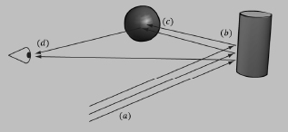
Figure 6.2: (a) Flux of incoming white light. (b) The light strikes the cylinder and some rays are absorbed and other rays are scattered toward the eye and the sphere. (c) The light reflecting off the cylinder toward the sphere is absorbed or reflected again and travels into the eye. (d) The eye receives incoming light that determines what the person sees.

According to the trichromatic theory (see [Santrock03]), the retina contains three kinds of colored light receptors, each sensitive to red, green, or blue light (with some overlap). The incoming RGB light stimulates its corresponding light receptors to varying intensities based on the strength of the light. As the light receptors are stimulated (or not), neural impulses are sent down the optic nerve toward the brain, where the brain generates an image in your head based on the stimulus of the light receptors. (Of course, if you close/cover your eyes, the receptor cells receive no stimulus and the brain registers this as black.)

For example, consider Figure 6.2 again. Suppose that the material of the cylinder reflects 75% red light and 75% green light and absorbs the rest, and the sphere reflects 25% red light and absorbs the rest. Also suppose that pure white light is being emitted from the light source. As the light rays strike the cylinder, all the blue light is absorbed and only 75% red and green light is reflected (i.e., a medium-high intensity yellow). This light is then scattered — some of it travels into the eye and some of it travels toward the sphere. The part that travels into the eye primarily stimulates the red and green cone cells to a semi-high degree; hence, the viewer sees the cylinder as a semi-bright shade of yellow. Now, the other light rays travel toward the sphere and strike it. The sphere reflects 25% red light and absorbs the rest; thus, the diluted incoming red light (medium-high intensity red) is diluted further and reflected, and all of the incoming green light is absorbed. This remaining red light then travels into the eye and primarily stimulates the red cone cells to a low degree. Thus the viewer sees the sphere as a dark shade of red.

The lighting models we (and most real-time applications) adopt in this book are called local illumination models. With a local model, each object is lit independently of another object, and only the light directly emitted from light sources is taken into account in the lighting process (i.e., light that has bounced off other scene objects to strike the object currently being lit is ignored). Figure 6.3 shows a consequence of this model.

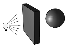
Figure 6.3: Physically, the wall blocks the light rays emitted by the light bulb and the sphere is in the shadow of the wall. However, in a local illumination model, the sphere is lit as if the wall were not there.

On the other hand, global illumination models light objects by taking into consideration not only the light directly emitted from light sources, but also the indirect light that has bounced off other objects in the scene. These are called global illumination models because they take everything in the global scene into consideration when lighting an object. Global illumination models are generally prohibitively expensive for real-time games (but come very close to generating photorealistic scenes); however, there is research being done in real-time global illumination methods.

6.2 Normal Vectors

A face normal is a unit vector that describes the direction a polygon is facing (i.e., it is orthogonal to all points on the polygon), as shown in Figure 6.4a. A surface normal is a unit vector that is orthogonal to the tangent plane of a point on a surface, as shown in Figure 6.4b. Observe that surface normals determine the direction a point on a surface is “facing.”

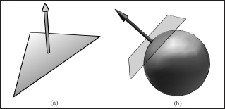
Figure 6.4: (a) The face normal is orthogonal to all points on the face. (b) The surface normal is the vector that is orthogonal to the tangent plane of a point on a surface.

For lighting calculations, we need to find the surface normal at each point on the surface of a triangle mesh so that we can determine the angle at which light strikes the point on the mesh surface. To obtain surface normals, we specify the surface normals only at the vertex points (so-called vertex normals). Then, in order to obtain a surface normal approximation at each point on the surface of a triangle mesh, these vertex normals will need to be interpolated across the triangle during rasterization (recall §5.9.3 and see Figure 6.5).

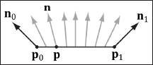
Figure 6.5: The vertex normals n₀ and n₁ are defined at the segment vertex points p₀ and p₁. A normal vector n for a point p in the interior of the line segment is found by linearly interpolating (weighted average) between the vertex normals; that is, n = n₀ + t(n₁ – n₀), where t is such that p = p₀ + t(p₁ – p₀). Although we illustrated normal interpolation over a line segment for simplicity, the idea straight-forwardly generalizes to interpolating over a 3D triangle.

6.2.1 Computing Normal Vectors

To find the face normal of a triangle Δp₀ p₁ p₂ we first compute two vectors that lie on the triangle’s edges:

u = p₁ – p₂

v = p₂ – p₀

Then the face normal is:

Below is a function that computes the face normal of the front side (§5.9.2) of a triangle from the three vertex points of the triangle.

For a differentiable surface, we can use calculus to find the normals of points on the surface. Unfortunately, a triangle mesh is not differentiable. The technique that is generally applied to triangle meshes is called vertex normal averaging. The vertex normal n for an arbitrary vertex v in a mesh is found by averaging the face normals of every polygon in the mesh that shares the vertex v. For example, in Figure 6.6, four polygons in the mesh share the vertex v; thus, the vertex normal for v is given by:

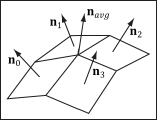
Figure 6.6: The middle vertex is shared by the neighboring four polygons, so we approximate the middle vertex normal by averaging the four polygon face normals.

In the above example, we do not need to divide by 4, as we would in a typical average, since we normalize the result. Note also that more sophisticated averaging schemes can be constructed; for example, a weighted average might be used where the weights are determined by the areas of the polygons (e.g., polygons with larger areas have more weight than polygons with smaller areas).

The following pseudocode shows how this averaging can be implemented given the vertex and index list of a triangle mesh:

6.2.2 Transforming Normal Vectors

Consider Figure 6.7a, where we have a tangent vector u = v₁ – v₀ orthogonal to a normal vector n. If we apply a nonuniform scaling transformation A, we see from Figure 6.7b that the transformed tangent vector uA = v₁A – v₀A does not remain orthogonal to the transformed normal vector nA.

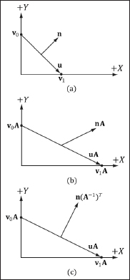
Figure 6.7: (a) The surface normal before transformation. (b) After scaling by 2 units on the x-axis the normal is no longer orthogonal to the surface. (c) The surface normal correctly transformed by the inverse-transpose of the scaling transformation.

So our problem is this: Given a transformation matrix A that transforms points and vectors (non-normal), we want to find a transformation matrix B that transforms normal vectors such that the transformed tangent vector is orthogonal to the transformed normal vector (i.e., uA · nB = 0). To do this, let’s first start with something we know: We know that the normal vector n is orthogonal to the tangent vector u.

u · n = 0	Tangent vector orthogonal to normal vector
un T = 0	Rewriting the dot product as a matrix multiplication
u(AA–)nT = 0	Inserting the identity matrix I = AA–1
(uA)(A–1n T) = 0	Associative property of matrix multiplication
(uA)((A–1n T)T)T = 0	Transpose property (AT)T = A
(uA)(n(A–1)T)T = 0	Transpose property (AB)T = BTAT
uA · n(A–1)T = 0	Rewriting the matrix multiplication as a dot product
uA ·nB = 0	Transformed tangent vector orthogonal to transformed normal vector

Thus B = (A –1)^T (the inverse-transpose of A) does the job in transforming normal vectors so that they are perpendicular to the associated transformed tangent vector uA.

Note that if the matrix is orthogonal (A^T = A^–1), then B = (A^–1)T = (A^T)^T = A; that is, we do not need to compute the inverse-transpose, since A does the job in this case. In summary, when transforming a normal vector by a nonuniform or shear transformation, use the inverse-transpose.

 

Note:    In this book, we only use uniform scaling and rigid body transformations to transform normals, so using the inverse-transpose is not necessary.

 

Note:    Even with the inverse-transpose transformation, normal vectors may lose their unit length; thus, they may need to be renormalized after the transformation.

6.3 Lambert’s Cosine Law

Light that strikes a surface point head-on is more intense than light that just glances a surface point (see Figure 6.8).

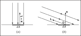
Figure 6.8: Consider a small area element dA. (a) The area dA receives the most light when the normal vector n and light vector L are aligned. (b) The area dA receives less light as the angle θ between n and L increases (as depicted by the light rays that miss the surface dA).

So the idea is to come up with a function that returns different intensities based on the alignment of the vertex normal and the light vector. (Observe that the light vector is the vector from the surface to the light source; that is, it is aimed in the opposite direction the light rays travel.) The function should return maximum intensity when the vertex normal and light vector are perfectly aligned (i.e., the angle θ between them is 0°), and it should smoothly diminish in intensity as the angle between the vertex normal and light vector increases. If θ > 90°, then the light strikes the back of a surface and so we set the intensity to 0. Lambert’s cosine law gives the function we seek, which is given by

f (θ) = max(cosθ, 0) = max(L · n, 0)

where L and n are unit vectors. Figure 6.9 shows a plot of f(θ) to see how the intensity, ranging from 0.0 to 1.0 (i.e., 0% to 100%), varies with θ.

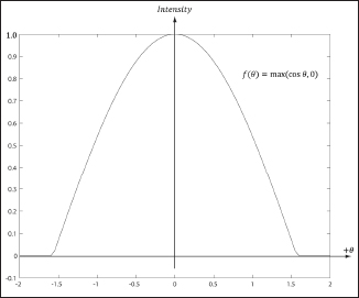
Figure 6.9: Plot of the function f(θ) = max(cos θ, 0) = max(L · n, 0)for –2 ≤ θ ≤ 2. Note that π/2 ≈ 1.57.

 

6.4 Diffuse Lighting

Consider a rough surface, as in Figure 6.10. When light strikes a point on such a surface, the light rays scatter in various random directions; this is called a diffuse reflection. In our approximation for modeling this kind of light/surface interaction, we stipulate that the light scatters equally in all directions above the surface; consequently, the reflected light will reach the eye no matter the viewpoint (eye position). Therefore, we do not need to take the viewpoint into consideration (i.e., the diffuse lighting calculation is viewpoint independent), and the color of a point on the surface will always look the same no matter the viewpoint.

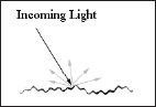
Figure 6.10: Incoming light scatters in random directions when striking a diffuse surface. The idea is that the surface is rough at a microscopic level.

We break the calculation of diffuse lighting into two parts. For the first part, we specify a diffuse light color and a diffuse material color. The diffuse material specifies the amount of incoming diffuse light that the surface reflects and absorbs; this is handled with a componentwise color multiplication. For example, suppose some point on a surface reflects 50% incoming red light, 100% green light, and 75% blue light, and the incoming light color is 80% intensity white light. Hence the incoming diffuse light color is given by c_D = (0.8, 0.8, 0.8) and the diffuse material color is given by m_D = (0.5, 1.0, 0.75); then the amount of light reflected off the point is given by:

c_D ⊗ m_D = (0.8, 0.8, 0.8) ⊗ (0.5, 1.0, 0.75) = (0.4, 0.8, 0.6)

 

Note:    The diffuse material may vary over the surface; that is, different points on the surface may have different diffuse material values. For example, consider a terrain mix of sand, grass, dirt, and snow; each of these terrain components reflects and absorbs light differently, and so the material values would need to vary over the surface of the terrain. In our Direct3D lighting implementation, we handle this by specifying a diffuse material value per vertex. These per-vertex attributes are then interpolated across the triangle during rasterization. In this way, we obtain a diffuse material value for each point on the surface of the triangle mesh.

To finish the diffuse lighting calculation, we simply include Lambert’s cosine law (which controls how much of the original light the surface receives based on the angle between the surface normal and light vector). Let c_D be the diffuse light color, m_D be the diffuse material color, and k_D = max(L · n, 0), where L is the light vector and n is the surface normal. Then the amount of diffuse light reflected off a point is given by:

6.5 Ambient Lighting

As stated earlier, our lighting model does not take into consideration indirect light that has bounced off other objects in the scenes. However, much of the light we see in the real world is indirect. For example, a hallway connected to a room might not be in the direct line of sight with a light source in the room, but the light bounces off the walls in the room and some of it may make it into the hallway, thereby lightening it up a bit. As a second example, suppose we are sitting in a room with a teapot on a desk and there is one light source in the room. Only one side of the teapot is in the direct line of sight of the light source; nevertheless, the back side of the teapot would not be pitch black. This is because some light scatters off the walls or other objects in the room and eventually strikes the back side of the teapot.

To sort of hack this indirect light, we introduce an ambient term to the lighting equation:

c_A ⊗ m_A

The color c_A specifies the total amount of indirect (ambient) light a surface receives from a light source. The ambient material color m_A specifies the amount of incoming ambient light that the surface reflects and absorbs. All ambient light does is uniformly brighten up the object a bit — there is no real physics calculation at all. The idea is that the indirect light has scattered and bounced around the scene so many times that it strikes the object equally in every direction.

 

Note:    In our implementation, we require that m_A = m_D; for example, if the surface reflects red diffuse light, then it also reflects red ambient light. Some other implementations allow m_A to be different from m_D for greater flexibility.

Combining the ambient term with the diffuse term, our new lighting equation looks like this:

6.6 Specular Lighting

Consider a smooth surface, as shown in Figure 6.11. When light strikes such a surface, the light rays reflect sharply in a general direction through a cone of reflectance; this is called a specular reflection. In contrast to diffuse light, specular light might not travel into the eye because it reflects in a specific direction; the specular lighting calculation is viewpoint dependent. This means that as the position of the eye changes within the scene, the amount of specular light it receives will change.

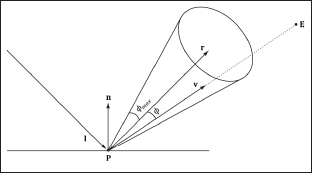
Figure 6.11: Specular reflections do not scatter in all directions, but instead reflect in a general cone of reflection whose size we can control with a parameter. If v is in the cone, the eye receives specular light; otherwise, it does not. The closer v is aligned with r, the more specular light the eye receives.

The cone the specular light reflects through is defined by an angle max with respect to the reflection vector r. Intuitively, it makes sense to vary the specular light intensity based on the angle ϕ between the reflected vector r and the view vector (i.e., the unit vector from the surface point P to the eye position E) in the following way: We stipulate that the specular light intensity is maximized when ϕ = 0 and smoothly decreases to 0 as ϕ approaches ϕmax. To model this mathematically, we modify the function used in Lambert’s cosine law. Figure 6.12 shows the graph of the cosine function for different powers of p ≥ 1 (i.e., p = 1, p = 8, and p = 128). Essentially, by choosing different values for p, we indirectly control the cone angle ϕmax where the light intensity drops to 0. The parameter p can be used to control the shininess of a surface; that is, highly polished surfaces will have a smaller cone of reflectance (the light reflects more sharply) than less shiny surfaces. So you would use a larger p for shiny surfaces than you would for matte surfaces.

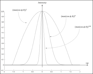
Figure 6.12: Plots of the cosine functions with different powers of p ≥ 1.

We now define the specular term of our lighting model:

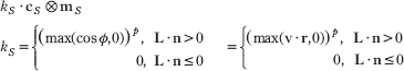
The color c_S specifies the amount of specular light the light source emits. The specular material color m_S specifies the amount of incoming specular light that the surface reflects and absorbs. The factor k_S scales the intensity of the specular light based on the angle between r and v. Figure 6.14 shows it is possible for a surface to receive no diffuse light (L · n < 0), but to receive specular light. However, if the surface receives no diffuse light, then it makes no sense for the surface to receive specular light, so we set k_S = 0 in this case.

 

Note:    The specular power p should always be ≥ 1.

Our new lighting model is:

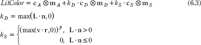
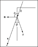
Figure 6.13: The eye can receive specular light even though the light strikes the back of a surface. This is incorrect, so we must detect this situation and set k_S = 0 in this case.

 

Note:    The reflection vector is given by r = I – 2(n · I)n (see Figure 6.14). (It is assumed that n is a unit vector.) However, we can actually use the HLSL intrinsic reflect function to compute r for us in a shader program.

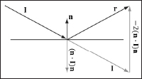
Figure 6.14: Geometry of reflection.

Observe that I, the incident vector, is the direction of the incoming light (i.e., opposite direction of the light vector L).

6.7 Brief Recap

In our model, a light source emits three different kinds of light:

     Ambient light: to model indirect lighting.

     Diffuse light: to model the direct lighting of relatively rough surfaces.

     Specular light: to model the direct lighting of relatively smooth surfaces.

Correspondingly, a surface point has the following material properties associated with it:

     Ambient material: the amount of ambient light the surface reflects and absorbs.

     Diffuse material: the amount of diffuse light the surface reflects and absorbs.

     Specular material: the amount of specular light the surface reflects and absorbs.

     Specular exponent: an exponent used in the specular lighting calculation, which controls the cone of reflectance and thus how shiny the surface is. The smaller the cone, the smoother/shinier the surface.

The reason for breaking lighting up into three components like this is for the flexibility; an artist has several degrees of freedom to tweak to obtain the desired output. Figure 6.15 shows how these three components work together.

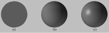
Figure 6.15: (a) Sphere colored with ambient light only, which uniformly brightens it. (b) Ambient and diffuse lighting combined. There is now a smooth transition from bright to dark due to Lambert’s cosine law. (c) Ambient, diffuse, and specular lighting. The specular lighting yields a specular highlight.

As mentioned in the Note in §6.4, we define material values at the vertex level. These values are then linearly interpolated across the 3D triangle to obtain material values at each surface point of the triangle mesh. Our vertex structure looks like this:

Recall that we have no ambient component because in our implementation we set m_A = m_D. Also, notice that we embed the specular power exponent p into the fourth component of the specular material color. This is because the alpha component is not needed for lighting, so we might as well use the empty slot to store something useful. The alpha component of the diffuse material will be used too — for alpha blending, as will be shown in a later chapter.

 

Note:    In some cases, large groups of vertices will share the same material values (see Figure 6.16), so it is wasteful to duplicate them. It may be more memory efficient to remove the material values from the vertex structure, sort the scene geometry into batches by material, set the material values in a constant buffer, and render like this pseudocode:

With this approach, the material information is fed into the shader programs through a constant buffer, rather than from the vertex data. However, this approach becomes inefficient if the batches are too small (there is some overhead in updating the constant buffer, as well as in Direct3D draw calls). A hybrid approach may be best: Use per-vertex materials when needed, and use constant buffer materials when they suffice. As always, you should customize the code based on your specific application requirements and the required trade-off between detail and speed.

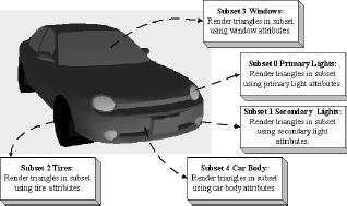
Figure 6.16: A car mesh divided into five material attribute groups.

Finally, we remind the reader that we need normal vectors at each point on the surface of a triangle mesh so that we can determine the angle at which light strikes a point on the mesh surface (for Lambert’s cosine law). In order to obtain a normal vector approximation at each point on the surface of the triangle mesh, we specify normals at the vertex level. These vertex normals will be interpolated across the triangle during rasterization.

Thus far we have discussed the components of light, but we have not discussed specific kinds of light sources. The next three sections describe how to implement parallel lights, point lights, and spotlights.

6.8 Parallel Lights

A parallel light (or directional light) approximates a light source that is very far away. Consequently, we can approximate all incoming light rays from this light as parallel to each other (see Figure 6.17). A parallel light source is defined by a vector, which specifies the direction the light rays travel. Because the light rays are parallel, they all use the same direction vector. The light vector aims in the opposite direction the light rays travel. A common example of a real directional light source is the Sun (see Figure 6.18).

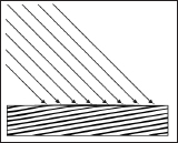
Figure 6.17: Parallel light rays striking a surface.

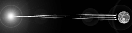
Figure 6.18: The figure is not drawn to scale, but if you select a small surface area on the Earth, the light rays from the Sun striking that area are approximately parallel.

6.9 Point Lights

A good physical example of a point light is a light bulb; it radiates spherically in all directions (see Figure 6.19). In particular, for an arbitrary point P, there exists a light ray originating from the point light position Q traveling toward the point. As usual, we define the light vector to go in the opposite direction; that is, the direction from point P to the point light source Q:

Essentially, the only difference between point lights and parallel lights is how the light vector is computed — it varies from point to point for point lights, but remains constant for parallel lights.

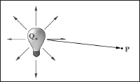
Figure 6.19: Point lights radiate in every direction; in particular, for an arbitrary point P there exists a light ray originating from the point source Q toward P.

6.9.1 Attenuation

Physically, light intensity weakens as a function of distance based on the inverse squared law. That is to say, the light intensity at a point a distance d away from the light source is given by:

where I₀ is the light intensity at a distance d = 1 from the light source. However, this formula does not always give aesthetically pleasing results. Thus, instead of worrying about physical accuracy, we use a more general function that gives the artist/programmer some parameters to control (i.e., the artist/programmer experiments with different parameter values until he is satisfied with the result). The typical formula used to scale light intensity is:

We call a₀, a₁, and a₂ attenuation parameters, and they are to be supplied by the artist or programmer. For example, if you actually want the light intensity to weaken with the inverse distance, then set a₀ = 0, a₁ = 1, and a₂ = 0. If you want the actual inverse square law, then set a₀ = 0, a₁ = 0, and a₂ = 1.

Incorporating attenuation into the lighting equation, we get:

6.9.2 Range

For point lights, we include an additional range parameter (see §6.11.1 and §6.11.3). A point whose distance from the light source is greater than the range does not receive any light from that light source. This parameter is useful for localizing a light to a particular area. Even though the attenuation parameters weaken the light intensity with distance, it is still useful to be able to explicitly define the max range of the light source. The range parameter is also useful for shader optimization. As we will soon see in our shader code, if the point is out of range, then we can return early and skip the lighting calculations with dynamic branching. The range parameter does not affect parallel lights, which model light sources very far away.

6.10 Spotlights

A good physical example of a spotlight is a flashlight. Essentially, a spotlight has a position Q, is aimed in a direction d, and radiates light through a cone (see Figure 6.20).

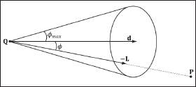
Figure 6.20: A spotlight has a position Q, is aimed in a direction d, and radiates light through a cone with angle ϕmax.

To implement a spotlight, we begin as we do with a point light. The light vector is given by:

where P is the position of the point being lit and Q is the position of the spotlight. Observe from Figure 6.20 that P is inside the spotlight’s cone (and therefore receives light) if and only if the angle ϕ between –L and d is smaller than the cone angle ϕmax. Moreover, all the light in the spotlight’s cone should not be of equal intensity; the light at the center of the cone should be the most intense and the light intensity should fade to 0 (zero) as ϕ increases from 0 to ϕmax.

So how do we control the intensity falloff as a function of ϕ, and how do we control the size of the spotlight’s cone? Well, we can play the same game we did with the specular cone of reflectance. That is, we use the function:

k_spot(ϕ) = (max(cos ϕ, 0))^S = (max(–L, · d, 0))^S

Refer back to Figure 6.12 for the graph of this function. As you can see, the intensity smoothly fades as ϕ increases, which is one of the characteristics we want; additionally, by altering the exponent s, we can indirectly control ϕmax (the angle the intensity drops to 0); that is to say, we can shrink or expand the spotlight cone by varying s. For example, if we set s = 8, the cone has approximately a 45° half angle.

So the spotlight equation is just like the point light equation, except that we multiply by the spotlight factor to scale the light intensity based on where the point is with respect to the spotlight cone:

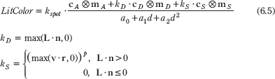
k_spot = (max(–L · d, 0))^S

6.11 Implementation

6.11.1 Lighting Structures

In an effect file, we define the following Light structure to represent either a parallel light, a point light, or a spotlight. Not all the members are used for each light.

    pos: The position of the light (ignored for directional lights).

    dir: The direction of the light (ignored for point lights).

    ambient: The amount of ambient light emitted by the light source.

    diffuse: The amount of diffuse light emitted by the light source.

    spec: The amount of specular light emitted by the light source.

    att: Stores the three attenuation constants in the format (a₀, a₁, a₂).

Attenuation constants are only applied to point lights and spotlights.

    spotPower: The exponent used in the spotlight calculation to control the spotlight cone; this value only applies to spotlights.

    range: The range of the light (ignored for directional lights).

This next structure (also defined in an effect file) stores the information at a surface point needed to light that point; that is, it stores the surface point itself, its normal, and the diffuse and specular material values at that point. At the moment, it matches our vertex structure (§6.7); however, our vertex structure is subject to change, but SurfaceInfo will not.

6.11.2 Implementing Parallel Lights

The following HLSL function outputs the lit surface color of Equation 6.3 given a parallel light source, the position of the eye, and the surface point information.

This code breaks Equation 6.3 down over several lines. The following intrinsic HLSL functions were used: dot, normalize, reflect, pow, and max, which are, respectively, the vector dot product function, vector normalization function, vector reflection function, power function, and maximum function. Descriptions of most of the HLSL intrinsic functions can be found in Appendix B, along with a quick primer on other HLSL syntax. One thing to note, however, is that when two vectors are multiplied with operator*, the multiplication is done componentwise.

6.11.3 Implementing Point Lights

The following HLSL function outputs the lit color of Equation 6.4 given a point light source, the position of the eye, and the surface point information.

6.11.4 Implementing Spotlights

The following HLSL function outputs the lit color of Equation 6.5 given a spotlight source, the position of the eye, and the surface point information.

Observe that a spotlight works just like a point light except that it is scaled based on where the surface point is with respect to the spotlight cone.

6.12 Lighting Demo

In our Lighting demo, we will have one light source active at a time. However, the user can change the active light by pressing one of the following keys: 1 (for parallel light), 2 (for point light), or 3 (for spotlight). The directional light remains fixed, but the point light and spotlight animate. The Lighting demo builds off the Waves demo from the previous chapter and uses the PeaksAndValleys class to draw a land mass, and the Waves class to draw a water mass. The effect file is given in §6.12.1, which makes use of the structures and functions defined in §6.11.

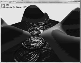
Figure 6.21: Screenshot of the Lighting demo.

6.12.1 Effect File

6.12.2 Structure Packing

The preceding effect file has a constant buffer with a Light instance. We would like to be able to set this value with one function call. Therefore, in the C++ code we define a structure very similar to the HLSL Light structure:

The issue with the “pad” variables is to make the C++ structure match the HLSL structure. In the HLSL, structure padding occurs so that elements are packed into 4D vectors, with the restriction that a single element cannot be split across two 4D vectors. Consider the following example:

If we have to pack the data into 4D vectors, you might think it is done like this:

However, this splits the element dir across two 4D vectors, which is not allowed — an element is not allowed to straddle a 4D vector boundary. Therefore, it has to be packed like this:

Thus, the “pad” variables in our C++ structure are able to correspond to those empty slots in the padded HLSL structure (since C++ does not follow the same packing rules as HLSL).

If we have a structure like this:

The structure would be padded and the data will be packed into three 4D vectors like so:

And a final example, the structure:

would be padded and packed like so:

6.12.3 C++ Application Code

In the application class, we have an array of three Lights, and also an integer that identifies the currently selected light by indexing into the light array:

They are initialized in the initApp method:

As mentioned, the point light and spotlight are animated; this is done in the updateScene method:

The point light basically follows a circular trajectory in the xz-plane, but always travels above the land or water. The spotlight is positioned at the eye and is aimed in the same direction the eye looks; this makes it look like the viewer is holding the light like a flashlight.

Finally, the selected light is set to the effect before rendering:

6.12.4 Normal Computation

Because our terrain surface is given by a function y = f(x, z), we can compute the normal vectors directly using calculus, rather than the normal averaging technique described in §6.2.1. To do this, for each point on the surface, we form two tangent vectors in the +x and +z directions by taking the partial derivatives:

These two vectors lie in the tangent plane of the surface point. Taking the cross product then gives the normal vector:

The function we use to generate the land mesh is:

f(x, z) = 0.3z · sin(0.1x)+ 0.3x· cos(0.1x)

The partial derivatives are:

The surface normal at a surface point (x, f(x, z), z) is thus given by:

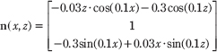
We note that this surface normal is not of unit length, so it needs to be normalized before performing the lighting calculations.

In particular, we do the above normal calculation at each vertex point to get the vertex normals:

The normal vectors for the water surface are done in a similar way, except that we do not have a formula for the water. However, tangent vectors at each vertex point can be approximated using a finite difference scheme (see [Lengyel02] or any numerical analysis book).

 

Note:    If your calculus is rusty, don’t worry; it will not play a major role in this book. Right now it is useful because we are using mathematical surfaces to generate our geometry so that we have some interesting objects to draw. Eventually, we will load 3D meshes from files that were exported from 3D modeling programs.

6.13 Summary

    With lighting, we no longer specify per-vertex colors but instead define scene lights and per-vertex materials. Materials can be thought of as the properties that determine how light interacts with a surface of an object. The per-vertex materials are interpolated across the face of the triangle to obtain material values at each surface point of the triangle mesh. The lighting equations then compute a surface color the eye sees based on the interaction between the light and surface materials; other parameters are also involved, such as the surface normal and eye position.

     A surface normal is a unit vector that is orthogonal to the tangent plane of a point on a surface. Surface normals determine the direction a point on a surface is “facing.” For lighting calculations, we need the surface normal at each point on the surface of a triangle mesh so that we can determine the angle at which light strikes the point on the mesh surface. To obtain surface normals, we specify the surface normals only at the vertex points (so-called vertex normals). Then, in order to obtain a surface normal approximation at each point on the surface of a triangle mesh, these vertex normals will be interpolated across the triangle during rasterization. For arbitrary triangle meshes, vertex normals are typically approximated via a technique called normal averaging. If the matrix A is used to transform points and vectors (non-normal vectors), then (A–¹)^T should be used to transform surface normals.

     A parallel (directional) light approximates a light source that is very far away. Consequently, we can approximate all incoming light rays as parallel to each other. A physical example of a directional light is the Sun relative to the Earth. A point light emits light in every direction. A physical example of a point light is a light bulb. A spotlight emits light through a cone. A physical example of a spotlight is a flashlight.

     Ambient light models indirect light that has scattered and bounced around the scene so many times that it strikes the object equally in every direction, thereby uniformly brightening it up. Diffuse light travels in a particular direction, and when it strikes a surface, it reflects equally in all directions. Diffuse light should be used to model rough and or matte surfaces. Specular light travels in a particular direction, and when it strikes a surface, it reflects sharply in one general direction, thereby causing a bright shine that can only be seen at some angles. Specular light should be used to model smooth and polished surfaces.

6.14 Exercises

1.    Modify the Lighting demo of this chapter so that the directional light only emits red light, the point light only emits green light, and the spotlight only emits blue light. Colored lights can be useful for different game moods; for example, a red light might be used to signify emergency situations.

2.    Modify the Lighting demo of this chapter by changing the specular power material component, which controls the “shininess” of the surface. Try p = 8, p = 32, p = 64, p = 128, p = 256, and p = 512.

3.    One characteristic of “toon” lighting (cartoon styled lighting) is the abrupt transition from one color shade to the next (in contrast with a smooth transition) as shown in Figure 6.22. This can be implemented by computing k_d and k_s in the usual way (Equation 6.5), but then transforming them by discrete functions like the following before using them in the pixel shader:

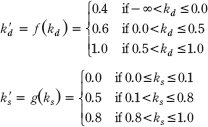
Modify the Lighting demo of this chapter to use this sort of toon shading. (Note: The functions f and g above are just sample functions to start with, and can be tweaked until you get the results you want.)

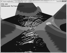
Figure 6.22: Screenshot of the toon shader.

4.    Modify the Lighting demo of this chapter to use one point light and one spotlight. Note that light is just summed together; that is, if c₁ is the lit color of a surface point from one light source and c₂ is the lit color of a surface point from another light source, the total lit color of the surface point is c₁ + c₂.

5.    Modify the Lighting demo of this chapter so that the angle of the spotlight’s cone can be increased or decreased based on the user’s keyboard input.